OLTP vs OLAP: A Complete Guide to How Databases Handle Transactions and Analytics
Every app that takes your order and every dashboard that reports your company’s sales depend on databases — but not the same kind of database, and not for the same reason. This guide breaks down exactly why, from first principles to production architecture, with worked examples from Amazon, Netflix, Uber, Swiggy, Flipkart and the Indian banking sector.
Introduction & History
Imagine two very different jobs happening inside a supermarket. The first is the cashier at the billing counter — scanning items, calculating your total, updating stock, and printing a receipt in two seconds. The second is the head-office analyst, sitting with a laptop, looking at six months of sales data across five hundred stores to figure out which product to discount next Diwali.
Both jobs involve the same underlying idea — “handling data” — but they are completely different in speed, size, and purpose. The cashier needs to process one transaction, instantly, correctly, every single time. The analyst needs to scan millions of past transactions and find patterns. Trying to make one system do both jobs equally well is like asking a sprinter to also run a marathon at sprint pace — it simply does not work efficiently.
This is exactly the difference between OLTP (Online Transaction Processing) and OLAP (Online Analytical Processing) — two categories of database systems, each engineered for one of these jobs.
Think of a busy restaurant kitchen. The order-taking counter is OLTP: waiters rush in one order at a time — “table 4 wants 2 dosas” — and the kitchen must confirm it instantly, update the order queue, and move to the next order. The restaurant owner reviewing a year of sales to decide “which dish should I remove from the menu because it barely sells” is OLAP: slow, thoughtful, working over huge piles of historical orders, not urgent to the second.
1.1 A short history
In the 1960s and 1970s, when computers first entered businesses (airlines, banks, and famously IBM’s early mainframe systems), the priority was simple: process one transaction — book one airline seat, withdraw money from one account — reliably and quickly. This gave rise to transaction processing systems, the ancestors of today’s OLTP databases. IBM’s System R and later commercial relational databases like Oracle (1979) and IBM DB2 were built with this transactional mindset, guided by the relational model that E. F. Codd proposed in 1970.
By the late 1980s and early 1990s, businesses had accumulated years of transactional data, and executives wanted to ask big-picture questions: “What were our total sales by region last quarter?” Running such heavy questions directly on the same database that was processing live customer transactions slowed everything down and sometimes crashed systems during busy hours. This need led to a new category of systems. In 1993, database pioneer E. F. Codd (again) published a paper coining the term OLAP, formalising the idea of a system purpose-built for multidimensional analysis. Companies began building separate data warehouses — large, dedicated stores optimised purely for analysis, decoupled from the live transactional systems.
Today, this split is a foundational pattern in system design. Nearly every serious production system — from Amazon’s checkout flow to Netflix’s recommendation engine — separates its “fast, live, transactional” data path from its “slow, historical, analytical” data path.
The OLTP vs OLAP distinction is one of the most frequently tested system-design fundamentals in software-engineering interviews, and it underlies real architectural decisions — choosing the wrong type of database for the wrong job is one of the most common and costly mistakes in production systems.
A useful piece of context: the two ideas did not emerge in isolation. OLTP grew out of the operational needs of banking, airline reservation and inventory systems, where correctness of every single transaction was existentially important. OLAP grew out of the analytical needs of business intelligence teams, who kept asking questions that operational databases were never designed to answer. Each category has since evolved its own culture, tooling, and even hiring pipelines — “application database engineer” and “data warehouse engineer” are often distinct roles at large companies today, precisely because the mental models required are so different.
The Problem & Motivation
To understand why OLTP and OLAP exist as separate categories, we need to understand what actually happens when you try to use a single database for both jobs.
2.1 Scenario — one database, two masters
Suppose an e-commerce company like Flipkart uses just one big database for everything: it stores every live order as customers buy things, and the same database also runs the monthly “total revenue by category” report for management. Here is what goes wrong:
- Heavy reports slow down live orders. A report that scans 50 million past rows to compute a sum can lock resources and slow down the simple “insert new order” queries happening at the same time. Customers experience a slow, laggy checkout page.
- Different data shapes are needed. Live orders need to be looked up by exact ID — “get order #4521” — extremely fast. Reports need to scan and group huge ranges of rows — “sum all orders from Karnataka in Q3.” The internal storage structure that makes one fast makes the other slow.
- Different scale of data. A transactional database might only need to keep “active” data — recent orders, current inventory. An analytical system often needs years of historical data, which is enormous by comparison.
- Different consistency needs. A transaction must never be half-done — you cannot charge a customer’s card without confirming their order. But a report reading data from five minutes ago instead of five seconds ago is usually perfectly fine.
A very common early-career mistake is running heavy analytical SQL queries — like monthly revenue aggregations — directly against the production transactional database during peak hours. This has caused real production outages at companies of every size because the reporting query locks rows or consumes so much CPU/I-O that live customer transactions time out.
The solution the industry converged on: build two specialised systems, each excellent at one job, and move data between them in a controlled way. That’s the essence of OLTP vs OLAP.
2.2 A concrete walkthrough
Let’s make this even more concrete with numbers. Imagine an Indian food-delivery company with 10 million orders placed every month. Each order insert touches maybe 4-5 rows: the order itself, order items, a payment record, and an inventory update. That single insert should complete in a few milliseconds, because a hungry customer is staring at a spinning loader on their phone.
Now imagine the finance team asks: “Show me total revenue, broken down by city and by week, for the last 18 months, along with the average order value.” To answer that question truthfully, the system must look through roughly 180 million historical order rows, group them by two different dimensions (city and week), and compute sums and averages. If you tried to run that query on the exact same database and tables used for live checkout — using row-by-row storage meant for single-record lookups — the database engine would have to read almost the entire table from disk, one row at a time, competing for the same CPU and I/O resources that live checkout traffic needs. On a large enough table, this single query could take many minutes — or hours — and during that time, ordinary checkout requests waiting on the same disk and CPU resources would slow down or time out.
This is precisely the scenario that pushed the industry toward maintaining two separate, purpose-built systems: one tuned for “microseconds per tiny operation, thousands of times per second” (OLTP), and another tuned for “seconds to minutes per huge operation, run occasionally” (OLAP).
Core Concepts
3.1 What is OLTP?
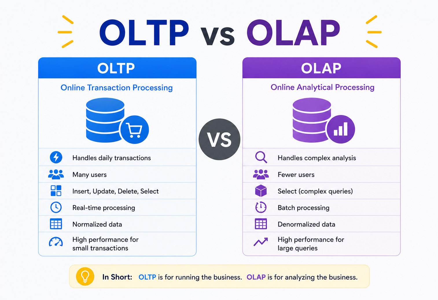
OLTP (Online Transaction Processing) refers to systems designed to manage large numbers of short, fast, real-time transactions — inserts, updates, deletes, and simple lookups — typically involving a small number of rows per operation.
Why it exists
Businesses need to record everyday operational events (a purchase, a bank transfer, a seat booking) instantly and reliably, with guarantees that the data is never left in a half-completed, inconsistent state.
Where it’s used
Banking apps, e-commerce checkout, airline booking systems, ATM withdrawals, food-delivery order placement, hospital patient record updates, ticket booking (IRCTC, BookMyShow).
OLTP is like a bank teller counter. One customer at a time, one specific request (“deposit ₹5,000 into account 1234”), completed fully and correctly before moving to the next customer.
Beginner example: When you tap “Buy Now” on Amazon, an OLTP system runs a transaction that (a) checks if the item is in stock, (b) reduces the stock count by one, (c) creates an order record, and (d) charges your payment method — all atomically, meaning either all four steps succeed, or none of them do.
-- A tiny, typical OLTP query: fetch ONE customer's ONE order
SELECT order_id, status, total_amount
FROM   orders
WHERE  order_id = 458213;

-- A typical OLTP write: update ONE row
UPDATE inventory
SET    stock_count = stock_count - 1
WHERE  product_id  = 9981;
Production example: Uber’s ride-matching and trip-status system is OLTP — every “driver accepted,” “trip started,” “trip completed” event must be recorded instantly and correctly for exactly one ride, right now.
3.2 What is OLAP?
OLAP (Online Analytical Processing) refers to systems designed to run complex queries over huge volumes of historical data, usually aggregating (summing, averaging, counting) across millions or billions of rows, to support business intelligence and decision-making.
Why it exists
Businesses need to understand trends and patterns across time — “how did sales grow over the last three years by region and product category” — questions that require scanning enormous datasets, which would be far too slow and disruptive on a live transactional system.
Where it’s used
Business dashboards, financial reporting, sales trend analysis, machine-learning feature pipelines, fraud pattern analysis, executive decision-making tools, marketing analytics.
OLAP is like a librarian who, instead of handing you one book, is asked: “Tell me how many books on cooking were borrowed each month for the last five years, broken down by branch.” It requires flipping through huge stacks of borrowing records and summarising — a completely different kind of work than handing over one book.
Beginner example: A retail company’s finance team asks: “What was our total revenue per state for each month in the last two years?” This requires scanning potentially hundreds of millions of order rows and grouping them by state and month — a job OLAP systems are built for.
-- A typical OLAP query: aggregate MILLIONS of rows
SELECT
    state,
    DATE_TRUNC('month', order_date) AS month,
    SUM(total_amount)               AS revenue,
    COUNT(*)                        AS order_count
FROM   orders_fact
WHERE  order_date BETWEEN '2024-01-01' AND '2026-01-01'
GROUP BY state, DATE_TRUNC('month', order_date)
ORDER BY month, revenue DESC;
Production example: Netflix’s internal analytics platform, which studies what millions of users watched last month to decide which shows to promote or renew, is powered by OLAP-style systems (built on top of large-scale data warehouses).
3.3 The one-line difference
OLTP answers: “What is happening right now, for this one specific record?”
OLAP answers: “What has happened over time, across huge amounts of data?”
3.4 The “O” in both names — Online
Notice both names start with “Online.” This word is a leftover from an older era of computing when the alternative was batch processing — where you submitted a stack of punch cards and waited hours or overnight for a printed result. “Online” simply means the system responds interactively, while you wait, rather than in a scheduled overnight batch. OLTP is “online” in the sense of instant, live transactions. OLAP is “online” in the sense that an analyst can interactively explore data and get an answer in seconds rather than submitting a job and waiting until the next morning — even though OLAP queries are still much slower than OLTP queries.
3.5 Transactions vs analytical queries — a side-by-side look
It helps to see the two kinds of work laid out next to each other for the same underlying business — a bookstore.
| Question asked | System type | Rows touched | Expected speed |
|---|---|---|---|
| “Add 1 copy of Wings of Fire to cart 4521” | OLTP | 1–2 rows | < 10 ms |
| “Reduce stock of ISBN 9788172234980 by 1” | OLTP | 1 row | < 10 ms |
| “What is the current stock of ISBN 9788172234980?” | OLTP | 1 row | < 10 ms |
| “Which genre sold best each quarter in the last 3 years?” | OLAP | Millions of rows | Seconds – minutes |
| “Average delivery delay by city, month over month?” | OLAP | Millions of rows | Seconds – minutes |
Notice the pattern: OLTP questions almost always have a specific subject — one cart, one book, one customer. OLAP questions almost always have a “group by” hiding inside them — by genre, by quarter, by city — because the goal is to summarise behaviour across a population of records, not to look up one of them.
3.6 Why beginners confuse the two
A common source of confusion for students is thinking “OLTP uses SQL and OLAP doesn’t” or “OLTP is for small companies and OLAP is for big companies.” Neither is true. Both categories are commonly queried using SQL. And even a small startup with a modest user base often benefits from separating a lightweight reporting database from its live application database once reports start taking noticeably long or slowing down the app — the size of the company doesn’t decide this, the shape and volume of the queries does.
Architecture & Components
OLTP and OLAP systems are architected fundamentally differently, because they optimise for opposite access patterns.
4.1 OLTP architecture
- Row-oriented storage: Data is stored row by row on disk, so that fetching one entire record (all columns of one order) is a single fast read.
- Normalized schema: Data is broken into many small related tables (customers, orders, products, inventory) to avoid duplication and keep updates cheap and consistent — following normalisation rules (1NF, 2NF, 3NF).
- Indexes on primary keys: Optimised for point lookups (find exactly one row) using B-Tree indexes.
- Locking & concurrency control: Mechanisms like row-level locks and Multi-Version Concurrency Control (MVCC) ensure many users can safely read and write at the same time without corrupting data.
4.2 OLAP architecture
- Column-oriented storage: Data is stored column by column, so that scanning and summing just one column (e.g.
amount) across millions of rows is extremely fast, since you don’t need to read unrelated columns. - Denormalized schema: Data is often organised in a star schema or snowflake schema — a central “fact table” (e.g. sales) surrounded by “dimension tables” (e.g. time, product, region) — designed to make large aggregations fast and queries simple to write.
- Heavy pre-aggregation & indexing strategies: Techniques like materialised views, bitmap indexes, and columnar compression speed up scanning.
- Massively Parallel Processing (MPP): Query execution is split across many machines and cores simultaneously, since queries touch huge amounts of data.
4.3 Schema comparison — normalized vs star
| Aspect | OLTP | OLAP |
|---|---|---|
| Storage layout | Row-oriented | Column-oriented |
| Schema design | Normalised (3NF) | Denormalised (Star / Snowflake) |
| Typical query | Point lookup, small update | Aggregation over millions of rows |
| Indexing focus | Primary key / B-Tree | Columnar compression, bitmap, zone maps |
| Concurrency model | Row locks, MVCC | Mostly read-heavy, batch loads |
4.4 Why normalization makes sense for OLTP
Normalisation means splitting data into smaller related tables so that each fact is stored exactly once. For example, a customer’s address is stored once in a customers table, not copied into every single order row. Why does this matter for OLTP?
- Cheaper, safer updates: If a customer changes their address, you update it in exactly one place. If the address were duplicated across every order row, you’d need to update thousands of rows and risk some of them being missed (data becoming inconsistent).
- Smaller row size: Each order row only stores a reference (
customer_id) instead of the customer’s full name and address, keeping theorderstable lean and fast to write. - Referential integrity: Foreign-key constraints ensure you can never insert an order for a
customer_idthat doesn’t exist — the database enforces correctness automatically.
4.5 Why denormalization makes sense for OLAP
In an OLAP warehouse, the same “one fact, one place” rule would force every analytical query to join five, ten or fifteen tables together just to answer a simple question like “total revenue by city.” Each join is computationally expensive, especially over millions of rows. Instead, OLAP schemas intentionally duplicate some data (like storing the city name directly alongside each sales record, rather than just a reference) so that queries can read straight from a small number of wide, pre-joined tables. The extra storage space this costs is a small price to pay for queries that run in seconds instead of minutes. This is a deliberate, informed trade-off — not sloppy database design.
Normalisation is like keeping one Aadhaar card with your address, and every form you fill out just references your Aadhaar number. Denormalisation is like printing your full name and address directly on every single form, so whoever reads the form later doesn’t need to go looking up your Aadhaar record separately — convenient for the reader, but means more re-typing if your address ever changes.
Internal Working
5.1 How OLTP processes a transaction — the ACID guarantee
OLTP systems are built around a promise called ACID:
- Atomicity — a transaction either fully happens or doesn’t happen at all. If step 3 of 4 fails, everything rolls back.
- Consistency — a transaction moves the database from one valid state to another valid state (e.g. account balances always add up correctly).
- Isolation — concurrent transactions don’t interfere with each other’s intermediate states.
- Durability — once a transaction is confirmed (“committed”), it survives even a power failure, because it’s been written to durable storage.
Think of a bank transfer of ₹1,000 from Account A to Account B. Atomicity means: either both “subtract from A” and “add to B” happen, or neither happens — you never end up with money vanishing or duplicating. This is why ACID is non-negotiable for OLTP.
Internally, OLTP databases use a Write-Ahead Log (WAL): before changing actual data on disk, the database first writes a note describing the intended change to a log file. If the system crashes mid-operation, it replays this log on restart to recover to a consistent state. This is how durability is guaranteed even during power failures.
For concurrency, most modern OLTP databases (PostgreSQL, MySQL InnoDB) use MVCC (Multi-Version Concurrency Control): instead of always locking rows when someone reads them, the database keeps multiple versions of a row, so readers see a consistent snapshot without blocking writers, and writers don’t block readers. This dramatically improves throughput under heavy concurrent load.
5.2 Isolation levels — controlling how much transactions see each other
The “I” in ACID (Isolation) is not all-or-nothing — SQL defines several isolation levels that trade off correctness guarantees against performance:
- Read Uncommitted: A transaction can see another transaction’s uncommitted changes (“dirty reads”). Rarely used because it’s unsafe.
- Read Committed: A transaction only ever sees data that has been committed by others. This is the default in PostgreSQL and Oracle.
- Repeatable Read: Guarantees that if you read the same row twice within one transaction, you’ll see the same value both times. This is MySQL InnoDB’s default.
- Serializable: The strictest level — transactions behave as if they ran one after another, never interleaved. Safest, but slowest, so used only when correctness is absolutely critical (e.g. transferring money between accounts with complex business rules).
Think of isolation levels like how carefully two people editing the same shared spreadsheet coordinate with each other. “Read Uncommitted” is like peeking at someone’s screen mid-edit before they’ve saved. “Serializable” is like a strict rule that only one person can touch the sheet at a time, start to finish — safest, but slowest if many people need access.
5.3 Underlying data structures — B-Trees and LSM-Trees
Most traditional OLTP databases (PostgreSQL, MySQL, Oracle) store their indexes using a B-Tree (or B+Tree) — a balanced tree structure that keeps data sorted and allows searches, insertions, and range lookups in logarithmic time, roughly O(log n). This is why looking up “order #458213” among 500 million rows still takes only a handful of disk reads.
Some newer high-write-throughput OLTP-style databases (like Cassandra and RocksDB, often used behind services needing extremely high write volume) instead use a Log-Structured Merge-Tree (LSM-Tree). An LSM-Tree buffers incoming writes in memory (a “memtable”) and periodically flushes them to disk in sorted, immutable batches, merging them in the background. This trades a little bit of read complexity for extremely fast, sequential-disk-friendly write performance — useful for workloads dominated by huge volumes of writes, like IoT sensor ingestion or activity logging.
5.4 Java example — a simple OLTP transaction
// A typical OLTP-style transaction in Java using JDBC
public void transferMoney(Connection conn, long fromAcct, long toAcct, BigDecimal amount)
        throws SQLException {
    try {
        conn.setAutoCommit(false); // start transaction

        String debit = "UPDATE accounts SET balance = balance - ? WHERE account_id = ?";
        try (PreparedStatement ps = conn.prepareStatement(debit)) {
            ps.setBigDecimal(1, amount);
            ps.setLong(2, fromAcct);
            ps.executeUpdate();
        }

        String credit = "UPDATE accounts SET balance = balance + ? WHERE account_id = ?";
        try (PreparedStatement ps = conn.prepareStatement(credit)) {
            ps.setBigDecimal(1, amount);
            ps.setLong(2, toAcct);
            ps.executeUpdate();
        }

        conn.commit();       // both updates succeed together
    } catch (SQLException e) {
        conn.rollback();     // if anything fails, undo everything
        throw e;
    } finally {
        conn.setAutoCommit(true);
    }
}
Explanation: This code debits one account and credits another inside a single transaction boundary. If the credit step fails after the debit succeeded, rollback() undoes the debit too — this is Atomicity in action, implemented with a few lines of JDBC.
5.5 How OLAP processes a query — columnar scan & parallelism
OLAP systems don’t worry much about ACID transactions on writes, because they mostly deal with bulk-loaded, already-finalised historical data. Their internal focus is on making read-heavy, scan-heavy queries fast. Key techniques:
- Columnar compression: Since a column typically has repetitive or similar values (e.g. a
statecolumn has only ~30 unique Indian states), OLAP engines compress columns extremely efficiently, sometimes 10× or more. - Vectorized execution: Instead of processing one row at a time, the engine processes a “batch” (vector) of thousands of values from a column using CPU SIMD instructions, hugely speeding up aggregation.
- Partition pruning: Data is physically split (partitioned) by, say, date. A query for “last month’s sales” only reads that month’s partition, skipping everything else.
- Massively Parallel Processing (MPP): A single query is split into pieces executed simultaneously across many nodes, then results are merged (a “scatter-gather” pattern).
5.6 Java example — simulating a simple columnar aggregation
To make the columnar idea concrete, here’s a simplified Java snippet showing the conceptual difference between scanning rows versus scanning a single column to compute a sum. It’s a simplified illustration, not how a real OLAP engine’s internals work, but it shows why touching only the needed column is faster.
// Row-oriented style: must read every field of every row, even unused ones
class OrderRow {
    int    orderId;
    String customerName;
    String city;
    double amount;
}

double sumAmountsRowStyle(List<OrderRow> rows) {
    double total = 0;
    for (OrderRow row : rows) {
        total += row.amount; // customerName, city, orderId loaded into memory but unused
    }
    return total;
}

// Column-oriented style: only the "amount" column is ever touched
double sumAmountsColumnStyle(double[] amountColumn) {
    double total = 0;
    for (double amt : amountColumn) {
        total += amt;        // no wasted memory bandwidth on unrelated fields
    }
    return total;
}
Explanation: In the row-oriented version, even though we only care about amount, the CPU still has to load whole row objects (including unused strings) into memory as it iterates. In the column-oriented version, only the exact numbers needed are packed tightly together in an array, which is both smaller in memory and far friendlier to CPU cache and SIMD vectorised instructions — this is the essence of why real OLAP engines are so much faster at aggregation over huge datasets.
Data Flow & Lifecycle
In a real production system, OLTP and OLAP are not isolated islands — data flows from one to the other. Understanding this flow is essential for system-design interviews and real architecture work.
6.1 Step-by-step lifecycle
Capture
A user action (placing an order) triggers an OLTP write — fast, ACID-compliant, small.
Extract
Periodically (or continuously via Change Data Capture, CDC), new or changed rows are pulled out of the OLTP database.
Transform
Data is cleaned, reshaped into the star schema, deduplicated, and enriched (e.g. adding a “region” column by joining with a lookup table).
Load
Transformed data is loaded into the OLAP data warehouse.
Analyze
Analysts and dashboards query the warehouse — never the live OLTP system — for reports and insights.
Older systems ran ETL as a nightly batch job (data was up to 24 hours stale). Modern architectures increasingly use Change Data Capture (CDC) tools (like Debezium) that stream every row-level change from the OLTP database’s transaction log into the warehouse in near real-time, keeping analytics dashboards minutes — not a day — behind.
6.2 How CDC actually works
Remember the Write-Ahead Log (WAL) mentioned earlier — the file where an OLTP database records every change before applying it? CDC tools like Debezium attach to this log and read it continuously, the same way the database itself would during crash recovery. Every insert, update, and delete is captured as a small event (e.g. “order 458213 changed status from PENDING to SHIPPED”) and published onto a message stream — commonly Apache Kafka. Downstream consumers subscribe to this stream and apply the same changes into the OLAP warehouse, usually within seconds.
This approach has an important advantage over older “poll the database every hour and copy new rows” batch ETL: it puts almost zero extra query load on the live OLTP database, because it’s reading the log file, not running competing SQL queries against the tables themselves.
Think of CDC like a courier who reads the shopkeeper’s daily sales register as entries are written, and immediately radios each sale to the head office — instead of head office sending someone to physically re-count the entire shop’s inventory once a day.
6.3 Batch vs streaming — a quick comparison
| Aspect | Batch ETL | Streaming CDC |
|---|---|---|
| Data freshness | Hours to a day stale | Seconds to minutes stale |
| Load on OLTP system | Query-based, can be heavy | Log-based, very light |
| Complexity | Simpler to build and reason about | Requires streaming infrastructure (Kafka, connectors) |
| Typical use case | Daily / weekly business reports | Near-real-time dashboards, fraud detection |
Advantages, Disadvantages & Trade-offs
OLTP — Advantages
- Extremely fast for single-record operations.
- Strong consistency guarantees (ACID).
- Supports thousands of concurrent small transactions.
- Data integrity is enforced by design (foreign keys, constraints).
OLTP — Disadvantages
- Very slow for large aggregation queries.
- Normalised schema makes complex reporting queries need many joins.
- Not designed to hold years of historical data efficiently.
- Heavy analytical queries can degrade live transaction performance.
OLAP — Advantages
- Extremely fast for aggregations over huge datasets.
- Optimised for complex, multi-dimensional analysis.
- Scales to petabytes of historical data.
- Frees the live transactional system from reporting load.
OLAP — Disadvantages
- Not designed for single-row instant updates.
- Data is often stale by minutes to hours (not real-time).
- Requires an additional ETL / CDC pipeline to keep in sync.
- More storage cost due to denormalisation and duplication.
7.1 The core trade-off
This is fundamentally a trade-off between write optimisation and read / aggregation optimisation. You cannot have a single physical data layout that is simultaneously the fastest possible for “update one row” and the fastest possible for “scan and sum 500 million rows.” Choosing OLTP vs OLAP (or both, connected via a pipeline) is choosing which access pattern to optimise for.
7.2 The hidden cost — running two systems
It’s worth being honest about the cost side of this trade-off too. Maintaining both an OLTP system and an OLAP system means:
- More infrastructure to manage: two (or more) database systems to monitor, secure, back up, and keep patched.
- A pipeline to build and maintain: ETL / CDC jobs can fail, and someone needs to notice and fix them, or the warehouse silently goes stale.
- Data duplication: the same business fact (e.g. “order 458213 was for ₹1,200”) physically exists in at least two places, which means more storage cost and a small risk of the two falling out of sync if the pipeline has a bug.
- Team skill overhead: engineers need to understand both transactional database design and analytical / warehouse design, which are genuinely different skill sets.
This is exactly why very small applications often start with just one database and only introduce a separate OLAP system once the pain of slow reports or a struggling production database makes the added complexity clearly worth it. Good engineering is about matching the solution to the actual scale of the problem, not applying the “correct” textbook architecture on day one for a five-table hobby project.
Performance & Scalability
8.1 Scaling OLTP
OLTP systems typically scale using these approaches:
- Vertical scaling: adding more CPU / RAM to a single database server — simple, but has a ceiling.
- Read replicas: copies of the primary database that serve read-only queries, reducing load on the primary that handles writes.
- Sharding (horizontal partitioning): splitting data across multiple database instances by a key (e.g.
customer_idrange or hash), so each shard handles a fraction of total traffic. Used by companies like Instagram and Uber for their user and trip databases. - Connection pooling & caching: tools like PgBouncer and Redis reduce load by reusing connections and caching hot, frequently-read data.
8.2 Scaling OLAP
- Massively Parallel Processing (MPP) clusters: systems like Amazon Redshift, Google BigQuery, and Snowflake distribute both storage and query execution across many nodes.
- Data partitioning: splitting large tables by date or region so queries only scan relevant partitions (“partition pruning”).
- Materialized views: pre-computed and stored aggregation results (e.g. “daily sales totals”) so repeat queries don’t need to recompute from scratch.
- Separation of storage and compute: modern cloud warehouses (Snowflake, BigQuery) store data cheaply on object storage and spin up compute clusters on demand, so you don’t pay for idle compute.
OLTP performance is measured in TPS (transactions per second) — how many small operations it can complete per second. OLAP performance is measured in query latency over large data volumes — how fast it can crunch through gigabytes or terabytes for one complex query.
8.3 A closer look at sharding
Sharding deserves a bit more explanation because it’s a frequent interview topic. Suppose a single OLTP database can comfortably handle 10,000 writes per second, but your application needs to handle 80,000 writes per second at peak (imagine a flash sale on Big Billion Days). One server, no matter how powerful, eventually hits a ceiling on disk I/O and CPU. Sharding splits the data — say, by customer_id % 8 — across 8 separate database instances, so each one only needs to handle roughly 10,000 writes per second, well within its comfortable range.
The trade-off: queries that need data from a specific customer are fast (you know exactly which shard to go to), but a query that needs to aggregate across all customers (like “total orders today across all customers”) now has to query all 8 shards and merge the results in the application layer — which starts to look a lot like the scatter-gather pattern used in OLAP systems. This is a good example of how, at large enough scale, OLTP systems borrow ideas from OLAP-style parallel processing.
8.4 A closer look at materialized views
A materialised view is the pre-computed, saved result of a query, stored physically like a table, and refreshed periodically (e.g. every 15 minutes or every night). If an OLAP dashboard shows “total sales per city today” and 500 different analysts open that dashboard throughout the day, recomputing the same expensive aggregation from scratch 500 times would be wasteful. Instead, the aggregation is computed once, stored as a materialised view, and every dashboard view simply reads the small, pre-computed result — often in milliseconds instead of seconds.
High Availability & Reliability
OLTP High Availability is critical because downtime directly stops revenue — no one can place an order or transfer money. Common patterns:
- Primary-replica replication: a standby replica can be promoted to primary within seconds if the primary fails (failover).
- Synchronous vs asynchronous replication: synchronous replication guarantees zero data loss on failover but adds write latency; asynchronous is faster but risks losing the last few transactions during a crash.
- Multi-region deployments: critical financial systems often replicate across geographic regions to survive a full data-centre outage.
OLAP High Availability is generally less time-critical (a dashboard being unavailable for 10 minutes rarely stops business), but reliability of the underlying data pipeline matters a lot:
- Pipeline retries and idempotency: ETL jobs are designed to be safely re-run without duplicating data if a step fails midway.
- Data quality checks: automated validation (row counts, null checks, referential checks) before data is marked “ready” for analysts, to avoid reporting on broken data.
- Backfill capability: the ability to reprocess historical data if a bug is found in a transformation, without needing the original OLTP data to still exist unchanged.
9.1 CAP theorem connection
The CAP theorem states that a distributed system can only guarantee two of three properties during a network partition: Consistency, Availability, and Partition tolerance. OLTP systems handling money or bookings usually lean toward CP (consistency over availability) — they’d rather reject a transaction than risk an inconsistent balance. OLAP / analytics systems often lean toward AP (availability over strict consistency) — it’s fine if a dashboard is a few minutes stale, as long as it’s available.
Security
OLTP security focuses on protecting individual, often sensitive, live records:
- Row-level access control: a user should only see their own orders, not everyone’s — enforced via row-level security policies.
- Encryption at rest and in transit: especially critical for PII (personally identifiable information) and payment data (PCI-DSS compliance).
- SQL injection prevention: using parameterised queries (as shown in the Java example earlier) instead of string concatenation.
- Audit logging: recording who changed what and when, for compliance (e.g. banking regulations).
OLAP security focuses on protecting aggregated insights and controlling who can see which slices of business data:
- Data masking / anonymisation: removing or hashing PII (like customer names) before loading into the warehouse, since analysts usually only need aggregate patterns, not individual identities.
- Column-level and role-based access: a regional sales manager might see only their region’s data; a finance executive sees everything.
- Data governance & lineage tracking: knowing exactly where a number in a report came from and who can access it, especially important for GDPR / data-privacy compliance.
OLTP security is like a bank vault that only lets you open your own locker, even though the vault holds thousands of lockers. OLAP security is more like a research report that shows “average income by neighbourhood” — useful and safe to share broadly — while carefully making sure no single individual’s income can be reverse-engineered from the aggregated numbers.
A practical example: an e-commerce OLTP database stores full customer names, phone numbers, and delivery addresses because the delivery partner genuinely needs them. When that same order data is loaded into the analytical warehouse for a “which products are trending in Tier-2 cities” report, the ETL / CDC pipeline typically strips out or hashes the customer’s name and phone number, keeping only what’s needed for the analysis (city, product category, amount) — this is called data minimisation, a core principle in modern privacy regulations like India’s Digital Personal Data Protection Act and the EU’s GDPR.
Monitoring, Logging & Metrics
OLTP — Key Metrics
Transactions per second (TPS), query latency (p50 / p95 / p99), lock wait time, replication lag, connection-pool saturation, error / rollback rate.
OLAP — Key Metrics
Query execution time, data freshness (pipeline lag), ETL job success / failure rate, storage-and-compute cost per query, cache-hit ratio for materialised views.
Tools like Prometheus and Grafana are commonly used to monitor OLTP database health (connections, latency, replication lag), while data-pipeline observability tools (like Airflow’s UI, dbt’s run logs, or Monte Carlo for data quality) monitor the health and freshness of OLAP pipelines.
Deployment & Cloud
Modern cloud platforms offer purpose-built managed services for each category, so teams rarely build these from scratch anymore:
| Category | Popular products |
|---|---|
| OLTP (relational) | Amazon RDS (PostgreSQL / MySQL), Amazon Aurora, Google Cloud SQL, Azure SQL Database |
| OLTP (NoSQL, high-scale) | Amazon DynamoDB, MongoDB, Cassandra |
| OLAP (data warehouse) | Snowflake, Amazon Redshift, Google BigQuery, Azure Synapse |
| OLAP (open-source engines) | ClickHouse, Apache Druid, Apache Pinot, Presto / Trino |
A common modern pattern is the Lakehouse architecture (popularised by Databricks with Delta Lake, and also seen in Apache Iceberg and Hudi) — combining the low storage cost and flexibility of a data lake with the structured querying performance of a warehouse, blurring the old hard line between “data lake” and “data warehouse.”
ETL, Data Warehouses & Data Lakes
Since OLAP systems depend on data originating in OLTP systems, it’s worth understanding the surrounding ecosystem.
13.1 ETL vs ELT
ETL (Extract, Transform, Load): data is transformed before loading into the warehouse — the traditional approach, where transformation happens on a separate processing server.
ELT (Extract, Load, Transform): raw data is loaded first, and transformation happens inside the powerful warehouse itself using SQL — the modern approach enabled by cheap cloud compute (used by tools like dbt).
13.2 Data warehouse vs data lake vs data lakehouse
- Data Warehouse: stores structured, cleaned, schema-defined data — optimised for fast SQL analytics (the classic OLAP target).
- Data Lake: stores raw data of any format (structured, semi-structured, unstructured — logs, images, JSON) cheaply at massive scale, often on object storage like Amazon S3.
- Data Lakehouse: combines both — raw data-lake storage with warehouse-like structure, transactions, and fast querying layered on top.
OLAP is the query and processing style — the “how you ask questions of data.” Data warehouses and lakehouses are the storage systems that make OLAP-style queries fast. You’ll often hear these terms used together, but they answer different questions: OLAP = access pattern, warehouse / lakehouse = where the data lives.
Design Patterns & Anti-Patterns
14.1 Good patterns
- CQRS (Command Query Responsibility Segregation): separate the write model (OLTP-style, optimised for commands) from the read model (often OLAP-style or a denormalised read replica, optimised for queries) — a direct architectural embodiment of the OLTP / OLAP split at the application level.
- Change Data Capture (CDC) pipelines: stream row-level changes from OLTP into OLAP in near real-time instead of slow nightly batches.
- Read replicas for reporting: for smaller-scale needs, a read replica of the OLTP database (not the primary) can serve lightweight reporting queries without a full warehouse.
CQRS deserves a slightly deeper look because it’s a favourite in system-design interviews. In a typical CRUD application, the same database model handles both “write a new order” and “show me all orders for this customer, sorted by date, with product names filled in.” As the read side grows complex — needing joins, filters, and sorting the write model was never designed for — CQRS splits things: writes still go through a normalised, ACID-compliant OLTP model, but every write also updates a separate, denormalised read model (which could be a read replica, a search index like Elasticsearch, or even a small OLAP-style store) built specifically to answer read queries fast. The two models are kept in sync asynchronously, meaning reads might lag writes by a small amount — a trade-off very similar to the OLTP-to-OLAP lag we discussed earlier, just applied at a smaller, per-feature scale rather than across an entire company’s data warehouse.
14.2 Anti-patterns to avoid
Running a heavy monthly report query directly against the live primary database used for checkout is one of the most common production incidents. It locks resources and slows down real customer transactions. Always redirect analytical queries to a replica or a dedicated warehouse.
Applying strict 3NF normalisation (an OLTP habit) to a data warehouse leads to reports needing 15+ table joins, making them painfully slow. Warehouses should embrace denormalisation (star schema) intentionally.
Not clearly documenting how stale warehouse data can be (5 minutes? 24 hours?) leads to executives making decisions on outdated numbers without realising it. Always publish a freshness guarantee.
Best Practices & Common Mistakes
OLTP — Best Practices
- Keep transactions short and focused.
- Use proper indexing on frequently queried columns.
- Use connection pooling.
- Set up read replicas early for read-heavy workloads.
- Monitor and tune slow queries proactively.
OLAP — Best Practices
- Design the star schema around real business questions.
- Partition large tables by date.
- Use materialised views for frequently repeated aggregations.
- Automate data-quality checks in the pipeline.
- Document data freshness and lineage clearly.
15.1 Common mistakes engineers make early in their career
Having reviewed many production incidents over the years, a few mistakes come up again and again, especially among engineers who are new to thinking about OLTP and OLAP as distinct concerns:
- Adding a report feature directly to the main app database “just this once.” It starts as one small dashboard query and quietly grows into a dozen more, until the production database is silently overloaded during business hours — with no one having made a deliberate decision to build a full reporting system.
- Forgetting that a warehouse’s data can go stale silently. If a CDC or ETL pipeline breaks and no one is alerted, a dashboard can keep showing numbers from three days ago while looking perfectly normal — leading to decisions being made on outdated information without anyone realising it.
- Treating index creation as free. Every additional index speeds up reads but slows down writes (because the index itself must be updated on every insert or update). In write-heavy OLTP tables, adding too many indexes “just in case” can quietly hurt transaction throughput.
- Copying OLTP schema-design habits into a warehouse. Engineers who are only trained in OLTP-style normalisation sometimes build a warehouse with the same heavily normalised structure, not realising that a warehouse is meant to be queried very differently — resulting in painfully slow reports full of unnecessary joins.
Real-World Industry Examples
This “OLTP for the live product, OLAP for the business intelligence” pattern is close to universal across large-scale production systems, precisely because trying to merge the two leads to the performance and reliability problems discussed in Section 2.
FAQ
Can the same database technology be used for both OLTP and OLAP?
Some modern databases (like SingleStore, or PostgreSQL with columnar extensions) support Hybrid Transactional / Analytical Processing (HTAP), aiming to serve both patterns reasonably well in one system. However, at large scale, most production systems still separate them for the performance and isolation reasons discussed above.
Is OLAP always slower than OLTP?
Not “slower” in a bad sense — they measure different things. OLTP is fast at tiny operations (milliseconds per row). OLAP is fast at huge operations (seconds for billions of rows) — something that would take an OLTP system hours or crash it entirely.
Do small applications need a separate OLAP system?
Not necessarily. A small app with a few thousand rows can often run simple reports directly on its OLTP database without issues. The need for a separate OLAP system grows as data volume and reporting complexity increase — typically once reports start impacting live performance.
What does “real-time analytics” mean if OLAP is usually not instant?
Modern streaming OLAP engines (like Apache Druid or Apache Pinot) are specifically built to ingest data continuously and answer analytical queries within seconds of an event happening, narrowing the traditional gap. This is used for use cases like live fraud-detection dashboards.
Is NoSQL the same as OLTP, and SQL the same as OLAP?
No — this is a common misconception. OLTP and OLAP describe workload patterns, not specific technologies. NoSQL databases like MongoDB or DynamoDB are typically used for OLTP-style workloads, but SQL databases (like PostgreSQL) are also very commonly used for OLTP. Similarly, many OLAP engines use SQL as their query language.
How much data lag is “acceptable” between OLTP and OLAP?
It depends entirely on the business need. A monthly board report can tolerate a day of lag. A fraud-detection dashboard might need data within seconds. There is no universal correct answer — the right approach is to explicitly define a freshness SLA (Service Level Agreement) with stakeholders so everyone knows what “current” means for a given dashboard, rather than assuming it’s real-time by default.
As a beginner, which should I learn first — OLTP or OLAP concepts?
Start with OLTP. Almost every introductory database course, and almost every early-career backend engineering job, revolves around OLTP concepts — normalisation, ACID transactions, indexing, and basic SQL CRUD operations. Once you’re comfortable there, OLAP concepts (star schemas, aggregation, warehousing) build naturally on that foundation and become much easier to understand, because you’ll already know what problem they were invented to solve.
Summary & Key Takeaways
Key takeaways
- OLTP handles fast, small, real-time transactions (placing an order); OLAP handles large-scale historical analysis (total sales by region over 2 years).
- OLTP uses row-oriented, normalised storage for fast single-record reads and writes; OLAP uses column-oriented, denormalised (star schema) storage for fast aggregation.
- OLTP guarantees ACID properties for correctness; OLAP prioritises scan speed and typically tolerates slightly stale data.
- Data usually flows from OLTP into OLAP systems via ETL / ELT or Change Data Capture (CDC) pipelines.
- Running heavy analytical queries directly on a production OLTP database is a classic anti-pattern that causes real outages.
- Modern cloud platforms offer dedicated managed services for each: RDS / Aurora / DynamoDB for OLTP, Snowflake / BigQuery / Redshift for OLAP.
- Patterns like CQRS and Lakehouse architectures show how the OLTP / OLAP distinction shapes modern system design beyond just databases.
If you remember nothing else from this guide, remember this: OLTP and OLAP are not competing technologies where one is “better” than the other — they are two answers to two different questions. OLTP keeps the lights on for your live product, one small, correct transaction at a time. OLAP looks back across everything that has happened and turns it into insight the business can act on. Nearly every serious production system you’ll ever work on, from a college project database to a bank’s core systems, benefits from understanding when you’re solving an OLTP problem, when you’re solving an OLAP problem, and how to connect the two cleanly rather than forcing one system to awkwardly do both jobs at once.