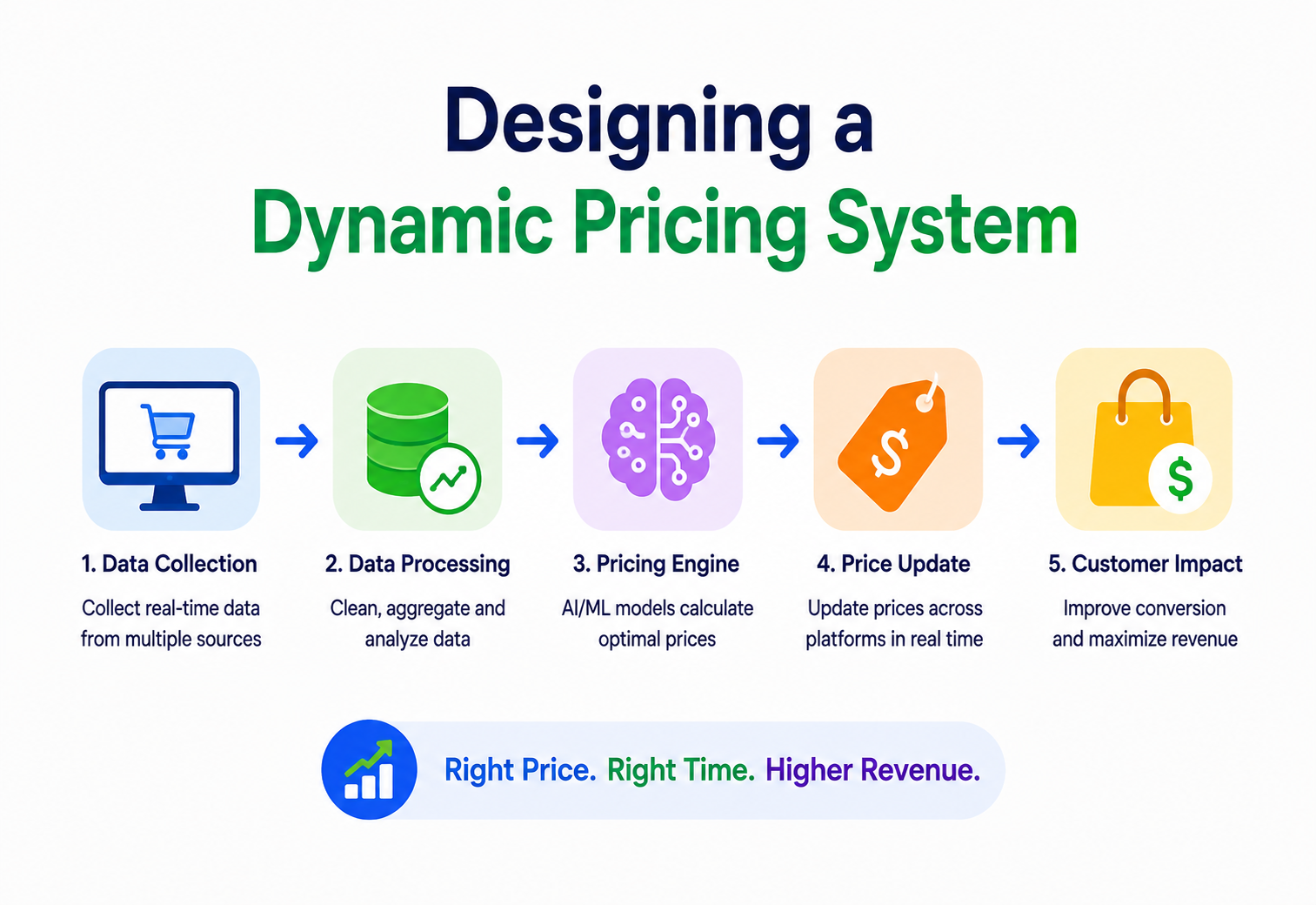
Designing a Dynamic Pricing System
A from-first-principles walkthrough of how large e-commerce and marketplace platforms adjust prices in near real time from demand, live inventory, and competitor pricing — architecture, data flow, scaling, reliability, and security.
Introduction and History
Open an airline booking page twice in the same afternoon and you may find two different fares for the exact same seat. Refresh a ride-hailing app on a rainy evening and the fare has jumped compared to an hour earlier. Browse a large online marketplace during a flash sale and the prices on competing sellers appear to shift almost by the minute. None of this is an accident, and none of it is a human sitting at a desk manually editing price tags. It is the output of a dynamic pricing system — a piece of software infrastructure that continuously recalculates the price of a product from live signals such as how many people want it right now, how much stock is left, and what competitors are charging.
Dynamic pricing is not a new idea. Airlines pioneered algorithmic fare management in the late 1970s and early 1980s, after industry deregulation in the United States forced carriers to compete directly on price for the first time. American Airlines built one of the earliest computerized “yield management” systems, which tried to sell the right seat to the right customer at the right price at the right time. Hotels followed with similar revenue management systems through the 1980s and 1990s, adjusting room rates based on occupancy forecasts and seasonal demand.
What changed everything was the arrival of large-scale e-commerce and, later, ride-hailing and food-delivery platforms. Unlike an airline that changes a few thousand fares a day, a large online retailer might carry tens of millions of distinct products (called SKUs, or stock-keeping units), each of which could theoretically need a new price every few minutes based on shifting demand, stock levels, and what dozens of competitors are charging for the same item. This is a fundamentally different scale of problem, and it is why dynamic pricing today is really a distributed-systems and data-engineering challenge as much as it is an economics one.
Picture a vegetable seller at an open-air market late in the day. As evening approaches, unsold tomatoes will spoil overnight, so the seller starts calling out lower prices to clear the stock. If a sudden crowd shows up because a nearby stall ran out of tomatoes, the same seller might raise the price slightly because demand just spiked. The seller is doing dynamic pricing in their head, using two signals: how much stock is left, and how much people want it right now. A software dynamic pricing system does the exact same thing, except across millions of products, thousands of times per second, using data instead of intuition.
By the mid-2010s, dynamic pricing had become a default expectation for any serious e-commerce platform, and this guide focuses squarely on that generation of systems: web-scale, near-real-time, and built on the same distributed-systems building blocks used everywhere else in modern backend engineering — API gateways, load balancers, message queues, caches, and machine learning services.
The Problem and Why Static Pricing Fails
Before designing anything, it helps to be precise about the problem. A traditional e-commerce catalog stores one price per product in a database table, and that price changes only when a human manually edits it, perhaps once a week during a planning meeting. This is called static pricing, and it breaks down badly at scale for several concrete reasons.
2.1 Demand is not constant
Interest in a product rises and falls throughout the day and across seasons. A static price is either too low during a demand spike — leaving money on the table and often causing the item to sell out and disappoint customers who arrive later — or too high during a demand lull, leaving inventory sitting unsold while it slowly loses value.
2.2 Inventory carries real cost and real risk
Every unit of unsold stock ties up warehouse space and working capital, and in the case of perishable or seasonal goods it risks becoming worthless. A system that can gently lower prices as inventory nears its expiry window, or as a season ends, converts stock into cash before it becomes a write-off.
2.3 Competitors move first
In any category with more than one seller, price is one of the strongest signals a shopper uses to decide where to buy. If a competitor drops their price on an identical product and a retailer does not respond within minutes or hours, that retailer quietly loses sales without ever knowing why. Waiting for a weekly pricing review to catch this is far too slow.
2.4 Manual pricing does not scale
A retailer with 50 products can price them by hand. A retailer with 50 million products, spread across thousands of categories, cannot. The only way to price a catalog of that size intelligently is to build a system that can evaluate demand, inventory, and competitor data automatically, at machine speed.
2.5 Slow reactions compound into lost trust
Beyond the direct revenue impact, there is a subtler cost to slow pricing. A shopper who repeatedly finds a better deal elsewhere, without the original retailer ever adjusting to stay competitive, gradually forms a habit of checking that other retailer first. By the time a pricing team notices the erosion in a quarterly report, the underlying behavior change in customers may already be well established and difficult to reverse. This is part of why the business case for dynamic pricing is rarely just “capture a bit more margin” — it is equally about defending market position against competitors who are already pricing dynamically.
Build a system that, for any product in a catalog of tens of millions of items, can compute a new price within seconds to a few minutes of a meaningful change in demand, inventory, or competitor price — while respecting business rules such as minimum margin, maximum daily price movement, and legal constraints — and can do this reliably, securely, and cheaply at very high request volume.
“Why can’t we just recompute prices with a nightly batch job instead of building a real-time system?” A strong answer explains that batch pricing is fine for slow-moving signals like seasonal trends, but demand spikes (a product going viral, a competitor flash sale, a stock-out) can happen within minutes, and a system that only reacts once a day will lose revenue or lose customers to competitors who react faster. The best real systems use a hybrid: batch jobs for slow signals like long-term demand forecasting, and streaming pipelines for fast signals like competitor price changes and stock-outs.
Core Concepts You Need First
Before looking at architecture diagrams, it helps to build a shared vocabulary. Each term below is explained in plain language, with why it exists and a simple example.
3.1 Price elasticity of demand
This measures how sensitive the quantity of a product sold is to a change in its price. If a 5% price increase causes demand to fall by 20%, the product is highly “elastic” — customers are price-sensitive and will switch to alternatives quickly. If demand barely moves even with a large price change, the product is “inelastic” — think of a life-saving medicine with no substitute. A pricing engine uses elasticity estimates to decide how aggressively it can raise or lower a price without hurting revenue.
Think of elasticity like a rubber band. A highly elastic product stretches (loses many buyers) the moment you pull on price. An inelastic product barely stretches at all, even under a strong pull.
3.2 Price floor and price ceiling
The floor is the lowest price a business is willing to sell at, usually set so it still covers cost plus a minimum margin. The ceiling is the highest price allowed, often set to avoid appearing exploitative or breaking a legal cap. Every automated pricing decision must be clamped between these two bounds before it is ever shown to a customer.
3.3 Demand signal
Any measurable piece of data that indicates how much people currently want a product: page views, add-to-cart events, completed purchases in the last few minutes, search volume, or even external signals like weather or trending social topics for seasonal goods.
3.4 Competitor price feed
A stream of prices for the same or similar products, gathered either through partnerships and licensed data feeds, or through automated web scraping of publicly available prices. This feed is one of the three central inputs to the pricing decision, alongside demand and inventory.
3.5 Repricing frequency
How often the system is allowed to change the price of a given product. Too frequent, and customers see prices “flicker” and lose trust; too infrequent, and the system reacts too slowly to real changes. Most production systems use a repricing window of anywhere from a few minutes to a few hours per product, sometimes varying this by category.
3.6 Guardrails and business rules
A set of hard constraints layered on top of the raw algorithmic output — for example, “never move price more than 10% in a single day,” or “never price below cost,” or “match but never undercut this specific competitor by law in certain regulated categories.” These rules exist to prevent an algorithm from making an embarrassing or even illegal pricing decision on its own.
| Term | What it answers | Typical data source |
|---|---|---|
| Demand signal | How much do people want this right now? | Clickstream events, search logs, cart events |
| Inventory level | How much stock is left, and how urgently must it move? | Warehouse management, order management |
| Competitor price | What are others charging for the same item? | Price feed partners, scraping pipelines |
| Elasticity model | How will demand react if we change price? | Historical sales data, ML model |
| Guardrails | What are we never allowed to do? | Business and legal policy configuration |
3.7 Base price versus effective price
Most systems distinguish between a base price, which is a relatively stable reference value set by a category manager or a cost-plus-margin formula, and the effective price, which is the base price after all of the dynamic multipliers and guardrails described in this guide have been applied. Keeping these as two separate, clearly named values matters enormously for debugging: whenever a price looks wrong, the very first question is whether the base price itself was set incorrectly, or whether the dynamic adjustment logic misbehaved on top of a perfectly reasonable base price. Conflating the two into a single mutable field makes that question far harder to answer after the fact.

3.8 Repricing horizon versus repricing trigger
It helps to separate two related but distinct ideas. The repricing horizon is the maximum amount of time a price is allowed to go without being reviewed, acting as a safety net — even a completely stable, slow-moving product should still be recomputed at least this often. A repricing trigger, by contrast, is an event that causes an immediate, out-of-cycle recomputation, such as a competitor price change crossing a meaningful threshold, or inventory dropping below a critical count. A mature system uses both together: the horizon guarantees a maximum staleness bound, while triggers allow the system to react faster than the horizon alone would permit when something significant happens.
3.9 Cold-start products
A newly listed product has no purchase history, which means the demand forecasting model has very little to work with — a situation commonly called the cold-start problem. Systems typically handle this by falling back to a category-level average elasticity and demand baseline borrowed from similar, already-established products, gradually shifting weight toward the new product’s own observed data as it accumulates enough views and sales to be statistically meaningful.
System Architecture and Components
With the vocabulary in place, here is the full picture. The diagram below shows every major component involved in taking a customer’s request for a product price, and separately, the background pipeline that continuously recalculates prices from demand, inventory, and competitor signals.
Below is what each labelled box in that diagram is actually responsible for, in plain terms.
CDN
Caches static assets (images, product page HTML shells) at edge locations close to the customer so the pricing request itself is the only thing that has to travel to the origin servers.
API Gateway
The single entry point for every client request. Handles authentication, applies per-client rate limiting, validates request shape, and routes traffic to the correct backend service.
Load Balancer
Distributes incoming requests across many identical instances of the Pricing Service using health checks, so no single server becomes a bottleneck or a single point of failure.
Pricing Service
The core service that, given a product ID, returns the current price. It first checks the cache, and only computes a fresh price when needed.
Rules Engine
Applies business guardrails such as price floors, ceilings, and maximum daily movement, after the raw algorithmic price has been produced.
Demand Forecast Service
A machine learning service that scores how demand is trending for a product using recent clickstream and sales data.
Inventory Service
Tracks real-time stock counts per warehouse or fulfillment center and exposes a “days of stock remaining” style signal.
Competitor Price Service
Ingests competitor prices from data feed partners or scraping pipelines and normalizes them for comparison against the internal catalog.
Redis Cache
Stores the current computed price for each product with a short time-to-live so read traffic almost never has to hit the database directly.
Price Database
The durable source of truth for the current and historical price of every product, typically a horizontally sharded relational or NoSQL store.
Kafka Event Bus
Carries demand events, inventory updates, and competitor price changes from producers to the stream processor and pricing services asynchronously.
Stream Processor
Continuously aggregates raw events into windowed metrics — for example, “add-to-cart count in the last five minutes” — that feed the pricing decision.
“Why do we need both an API Gateway and a Load Balancer — aren’t they the same thing?” No. The API Gateway operates at the application layer, handling authentication, request validation, and routing decisions across many different backend services (pricing, catalog, checkout). The Load Balancer typically sits behind or alongside it and is focused purely on distributing traffic across multiple instances of one specific service for scalability and fault tolerance. In many real deployments, the gateway itself uses a load balancer internally to reach service instances — the two are complementary layers, not substitutes.
4.1 Networking considerations
Every hop shown in the architecture diagram costs time, and that time adds up quickly in a system where the read path is expected to respond in well under a hundred milliseconds. Services within the Pricing Core and Data Layer typically communicate over a private virtual network, entirely isolated from the public internet, which both improves security and reduces latency compared to routing internal traffic out through a public endpoint and back in. Connection pooling is used heavily between the Pricing Service and its downstream dependencies — the cache, the database, and the Rules Engine — so that a new request does not pay the cost of establishing a fresh TCP and TLS connection on every call, which can easily dominate the latency budget for an otherwise fast operation. DNS-based service discovery, or a dedicated service mesh, lets each service find healthy instances of its dependencies dynamically as the fleet scales up and down, rather than relying on a static, manually maintained list of addresses that would quickly go stale.
4.2 Why the Load Balancer sits where it does
Placing the Load Balancer directly in front of the Pricing Service fleet, rather than in front of every individual downstream service, keeps the architecture easier to reason about: the Pricing Service becomes the single orchestration point that fans out to the Rules Engine, Demand Forecast Service, Inventory Service, and Competitor Price Service as needed, and each of those downstream services can have its own internal load balancing without the client or the API Gateway needing to know anything about their internal topology. This is an application of the general principle of encapsulating internal complexity behind a stable service boundary, which keeps the system easier to evolve over time as individual components are rearchitected.
Internal Working: How a Price Gets Computed
It helps to separate the system into two distinct paths that run at very different speeds: the read path, which serves a price to a customer in milliseconds, and the write path, which recomputes prices in the background every few minutes.
5.1 The read path — serving a price fast
When a customer opens a product page, the storefront calls the pricing API for that product’s current price. This must be extremely fast, because it happens on every single page view across the entire catalog. The Pricing Service almost never computes a price live in this path — instead, it looks up an already-computed price sitting in the Redis cache. If the cache has expired or was never populated (a “cache miss”), the service falls back to the Price Database, and repopulates the cache for next time.
5.2 The write path — recomputing prices in the background
This is where the real intelligence lives, and it runs continuously and independently of any single customer request. A simplified version of the core pricing formula many systems use looks like this:
new_price = base_price
          * demand_multiplier(demand_score)
          * inventory_multiplier(days_of_stock)
          * competitor_adjustment(competitor_price, base_price)

new_price = clamp(new_price, price_floor, price_ceiling)
new_price = apply_max_daily_move(new_price, previous_price, max_move_pct)
Each of the three multipliers pulls in one signal:
- Demand multiplier — increases price gently as recent demand (add-to-carts, purchases, searches) rises above a rolling baseline, and decreases it as demand falls below baseline.
- Inventory multiplier — decreases price as the “days of stock remaining” estimate drops toward zero for a fast-selling item that is nearly out, or, conversely, decreases price for slow-moving stock nearing an expiry or season-end date. A healthy stock level keeps this multiplier close to 1.0, meaning no adjustment.
- Competitor adjustment — nudges price toward a target position relative to the lowest tracked competitor price, for example “stay within 3% of the cheapest tracked competitor” as a business policy, without ever letting the price drop below the configured floor.
Here is a simplified Java implementation of that computation, written the way it might appear inside the Pricing Service.
public class PriceCalculator {

    private static final double MAX_DAILY_MOVE_PCT = 0.10;

    public BigDecimal computePrice(PricingContext ctx) {
        double demandMultiplier = demandMultiplier(ctx.getDemandScore());
        double inventoryMultiplier = inventoryMultiplier(ctx.getDaysOfStock());
        double competitorAdjustment = competitorAdjustment(
                ctx.getCompetitorPrice(), ctx.getBasePrice());

        BigDecimal rawPrice = ctx.getBasePrice()
                .multiply(BigDecimal.valueOf(demandMultiplier))
                .multiply(BigDecimal.valueOf(inventoryMultiplier))
                .multiply(BigDecimal.valueOf(competitorAdjustment));

        BigDecimal clamped = clamp(rawPrice, ctx.getFloor(), ctx.getCeiling());
        return applyMaxDailyMove(clamped, ctx.getPreviousPrice(), MAX_DAILY_MOVE_PCT);
    }

    private double demandMultiplier(double demandScore) {
        // demandScore is normalized between -1.0 (very low) and 1.0 (very high)
        return 1.0 + (demandScore * 0.08);
    }

    private double inventoryMultiplier(int daysOfStock) {
        if (daysOfStock <= 3) return 1.05;   // scarcity, small increase
        if (daysOfStock >= 60) return 0.92;  // overstock, discount to clear
        return 1.0;
    }

    private double competitorAdjustment(BigDecimal competitorPrice, BigDecimal basePrice) {
        if (competitorPrice == null) return 1.0;
        double ratio = competitorPrice.doubleValue() / basePrice.doubleValue();
        if (ratio < 0.97) return 0.98; // competitor notably cheaper, react
        return 1.0;
    }

    private BigDecimal clamp(BigDecimal price, BigDecimal floor, BigDecimal ceiling) {
        if (price.compareTo(floor) < 0) return floor;
        if (price.compareTo(ceiling) > 0) return ceiling;
        return price;
    }

    private BigDecimal applyMaxDailyMove(BigDecimal newPrice, BigDecimal previous, double maxPct) {
        BigDecimal upperBound = previous.multiply(BigDecimal.valueOf(1 + maxPct));
        BigDecimal lowerBound = previous.multiply(BigDecimal.valueOf(1 - maxPct));
        if (newPrice.compareTo(upperBound) > 0) return upperBound;
        if (newPrice.compareTo(lowerBound) < 0) return lowerBound;
        return newPrice;
    }
}Think of a thermostat. It does not redesign your heating system every time the room temperature changes by half a degree; it just nudges the output up or down within a safe range. The pricing engine works the same way — it nudges the price within floor and ceiling bounds rather than making wild, unbounded jumps.
“Where should the guardrail logic (floor, ceiling, max daily move) live — inside the same service that computes the raw price, or in a separate service?” Many production systems deliberately separate these into a distinct Rules Engine, even though it adds a network hop, because guardrails are a compliance and safety concern that product, legal, and finance teams need to change independently and audit separately from the machine-learning-driven pricing logic. Keeping them separate also means the guardrails can be applied uniformly regardless of which algorithm produced the raw price.
5.3 A complete worked example
It helps to walk through one concrete product end to end. Suppose a wireless headphone SKU has a base price of seventy dollars, a price floor of fifty-five dollars, and a ceiling of ninety-five dollars, with a maximum daily movement of ten percent. Over the last recomputation window, the demand signal came in strongly positive because the product started trending on social media, giving it a normalized demand score of 0.6. The inventory service reports twelve days of stock remaining at the current sales velocity, which is a healthy level, so the inventory multiplier stays neutral at 1.0. The competitor price feed shows the cheapest tracked competitor selling the same model for sixty-eight dollars, which is more than three percent below the base price, triggering the competitor adjustment multiplier.
Plugging these into the formula from earlier: the demand multiplier becomes 1.0 plus 0.6 times 0.08, which is 1.048. The inventory multiplier stays at 1.0. The competitor adjustment applies its 0.98 factor because the competitor is meaningfully cheaper. Multiplying these together against the seventy dollar base price gives a raw computed price of roughly seventy-one dollars and ninety cents. That value sits comfortably between the floor and ceiling, and is well within the ten percent daily movement allowance from whatever the previous price happened to be, so it passes through the Rules Engine unchanged and becomes the new published price. This same walkthrough, repeated automatically across the entire catalog on a rolling schedule, is the entire system in miniature.
“Walk me through what happens if two signals disagree — demand is spiking but a competitor just dropped their price sharply.” This is exactly the situation the multiplicative formula is designed to handle gracefully: each signal contributes its own independent multiplier, so a strong upward pull from demand and a strong downward pull from the competitor adjustment partially offset each other in the final raw price, rather than one signal being allowed to dominate arbitrarily. If the business wants one signal to matter more than another in certain categories, that is expressed by tuning the weight or sensitivity of that specific multiplier, not by special-casing the formula.
Algorithms, Data Structures and Concurrency
Underneath the service boundaries described so far, a handful of classical algorithms and data structures do most of the real work. Understanding these makes it much easier to reason about why the system behaves the way it does under load, and they come up frequently in system design interviews as follow-up questions once the high-level architecture has been sketched out.
6.1 Sliding and tumbling windows for demand aggregation
The Stream Processor needs to turn a firehose of individual events — an add-to-cart here, a purchase there — into a stable number like “demand this window.” Two windowing strategies are common. A tumbling window divides time into fixed, non-overlapping buckets, for example every five minutes, and aggregates each bucket independently; it is simple and cheap but can create a visible step change right at the window boundary. A sliding window instead maintains a continuously moving five-minute lookback, recalculated on every new event or on a short tick, which produces a smoother signal at the cost of more computation. Most production pricing pipelines use sliding windows for the demand signal specifically because customers are sensitive to abrupt price jumps, and a smoother input signal produces a smoother output price.
6.2 Count-min sketch for approximate demand counting
When a catalog has tens of millions of products, keeping an exact, precise counter for “events per product per window” in memory for every single product becomes expensive. Many large-scale pipelines instead use a probabilistic data structure called a count-min sketch, which trades a small, bounded amount of counting error for a dramatic reduction in memory usage — often orders of magnitude smaller than exact per-key counters. Since the pricing formula only needs a directionally correct demand score, not an exact count, this approximation is an excellent fit and is a common technique worth knowing for any high-cardinality counting problem, not just pricing.
6.3 Consistent hashing for cache and shard placement
Both the Redis cache layer and the sharded price database need a way to decide which node owns which product’s data, and to handle nodes being added or removed without reshuffling everything. Consistent hashing arranges nodes and keys on a conceptual ring using a hash function, so that adding or removing one node only affects the small slice of keys immediately adjacent to it on the ring, rather than requiring a full remap of every key in the system. This is the same technique used broadly across distributed caches and databases, and it is directly responsible for why the Pricing Service fleet can scale up or down without a painful, disruptive rebalance.
6.4 Priority queues for repricing scheduling
Not every product needs to be recomputed on the same fixed schedule. A practical implementation keeps a priority queue (often backed by a min-heap) of products ordered by “next scheduled recompute time.” Fast-moving, high-traffic products naturally bubble to the front of the queue more often, while long-tail products sit further back, giving the system a simple, efficient way to allocate limited compute budget where it matters most, in roughly logarithmic time per insertion or removal.
6.5 Concurrency control on the write path
Because multiple background jobs — a demand-triggered recompute, an inventory-triggered recompute, and a manual override — can all attempt to update the same product’s price at nearly the same time, the Pricing Service needs a concurrency control strategy to avoid lost updates. A common approach is optimistic concurrency control using a version number or timestamp column on the price record: a writer reads the current version, computes a new price, and writes it back only if the version has not changed in the meantime, retrying if it has. This avoids the throughput cost of holding a lock for the full duration of a computation, which matters because demand and competitor scoring can take tens of milliseconds and holding a database lock for that long across millions of products would be far too slow.
public class OptimisticPriceWriter {

    public boolean updatePrice(String productId, BigDecimal newPrice, long expectedVersion) {
        int rowsUpdated = priceRepository.updateIfVersionMatches(
                productId, newPrice, expectedVersion, expectedVersion + 1);
        return rowsUpdated == 1; // false means someone else updated first; caller should retry
    }
}Optimistic concurrency control is like editing a shared spreadsheet where each cell remembers the last time it was touched. Before saving your change, you check whether anyone else has touched that cell since you started editing. If they have, you re-read the latest value and redo your edit rather than blindly overwriting someone else’s work.
6.6 Example event payload
A representative demand event published to the Kafka bus, which the Stream Processor later aggregates into a windowed demand score, looks roughly like the structure below. Keeping the payload small and focused, rather than embedding the entire product catalog record into every event, keeps throughput high across a bus that may be carrying hundreds of thousands of these messages per second during peak traffic.
{
  "eventId": "evt-8f2a1c",
  "eventType": "ADD_TO_CART",
  "productId": "SKU-4471",
  "timestamp": "2026-07-30T09:14:22Z",
  "quantity": 1
}
6.7 Idempotency in the event pipeline
Message queues like Kafka generally offer at-least-once delivery, meaning the same demand or inventory event can occasionally be delivered more than once, especially after a consumer restart. The Stream Processor and Pricing Service must therefore be written so that processing the same event twice produces the same end state as processing it once — a property called idempotency. In practice this usually means keying aggregation state and price updates by a stable event identifier and checking whether that identifier has already been applied before mutating any counter or price.
“Two recompute jobs fire for the same product almost simultaneously — one triggered by a demand spike, one by an inventory update. How do you prevent them from clobbering each other’s results?” A strong answer reaches for optimistic concurrency control with a version check, explains why holding a distributed lock for the full computation would hurt throughput, and notes that on a version conflict, the losing job should simply re-read the latest state and recompute rather than failing outright, since the underlying signals it would recompute from have likely converged anyway.
Data Flow and Lifecycle
It is worth tracing a single price change from beginning to end, because this is a favorite whiteboard question in system design interviews. Two views are useful: the request-response sequence for a customer asking for a price, and the lifecycle a computed price object moves through before it is shown to anyone.
Separately, every candidate price a background job produces moves through its own lifecycle before it becomes the price customers actually see. This matters because a raw algorithmic output should never go straight to production without at least a validation step, and in many organizations, a manual or automated approval step for large price movements.
Notice the background pipeline is entirely event-driven. Demand events, inventory changes, and competitor price updates each arrive as messages on the Kafka bus. The Stream Processor consumes these messages in small time windows — for example, a five-minute tumbling window — and produces aggregated metrics such as “add-to-cart rate this window” or “current cheapest tracked competitor price.” Those aggregated metrics are what actually feed the Pricing Service’s next recomputation cycle, not the raw individual events, because acting on every single raw event would cause the price to change too often and too erratically.
Feeding raw, un-aggregated events directly into the pricing formula. This produces jittery prices that change every few seconds and confuse both customers and internal teams. Always aggregate over a window before it influences a live price.
7.1 Event schema and ordering guarantees
Each event on the Kafka bus carries a compact, versioned schema — a product identifier, an event type, a timestamp, and a small payload specific to that event type. Producers publish events keyed by product ID, which Kafka uses to guarantee that all events for the same product land in the same partition and are therefore processed in the order they were produced. This ordering guarantee matters because the Stream Processor’s windowed aggregation logic assumes events for a given product arrive in a roughly time-ordered sequence within a partition; without it, computing a rolling count or average over a time window would require much more complex out-of-order handling.
7.2 Backpressure and consumer lag
During an unusually large event burst — for instance, a viral moment driving a sudden flood of add-to-cart events for one product — the Stream Processor can temporarily fall behind the rate at which events are being produced. Kafka’s design tolerates this gracefully: events queue durably on the broker rather than being dropped, and the consumer catches up once the burst subsides, at the cost of a temporary increase in consumer lag, which is exactly why consumer lag is tracked as a first-class monitoring metric rather than an internal implementation detail.
Databases, Caching and Load Balancing
8.1 Choosing the price database
The price database is the durable source of truth. Because a large catalog can have tens of millions of SKUs, each needing frequent updates, this store is usually a horizontally partitioned (sharded) database, sharded by product ID or category. Many production systems use a wide-column or document store such as Cassandra or DynamoDB for this table specifically, because the access pattern is simple — read or write one row by product ID — and these stores scale write throughput linearly by adding more nodes, which a single relational instance cannot do as easily.
That said, a relational database with proper sharding (for example, using a tool like Vitess on top of MySQL) is also a very reasonable choice, especially if the organization already needs strong transactional guarantees around price changes for audit and compliance reasons.
8.2 Why caching is not optional
Consider a retailer serving 200,000 price lookups per second at peak. Sending every one of those requests to the database would require a database cluster large enough to sustain that read load continuously, which is expensive and fragile. Instead, the Pricing Service keeps the current price for every actively-viewed product in a Redis cache with a short time-to-live, typically somewhere between thirty seconds and a few minutes depending on how fresh prices need to be. This means the database only has to absorb the much smaller volume of actual price recomputations, not every customer read.
The cache is like a specials board at a restaurant, rewritten every hour from the kitchen’s records. Customers read the board, not the kitchen’s ledger, so a hundred customers can check prices without ever bothering the kitchen staff.
8.3 Cache invalidation strategy
Because the write path knows exactly when a price changes, the cleanest approach is write-through invalidation: the moment the Pricing Service publishes a newly approved price, it writes that price into Redis immediately, rather than waiting for the old cached value to expire naturally. The TTL still exists as a safety net in case an invalidation message is ever lost.

8.4 Load balancing across pricing instances
The Pricing Service typically runs as a fleet of many stateless instances behind a Layer 7 load balancer. Because each instance holds no session state — it only reads from cache and database — any instance can serve any request, which makes it trivial to add or remove instances as traffic changes. Health checks let the load balancer stop routing traffic to an instance that is failing, without any manual intervention.
| Layer | Technology examples | Why it fits here |
|---|---|---|
| Hot price cache | Redis, Memcached | Sub-millisecond reads, TTL support, huge throughput |
| Price source of truth | Cassandra, DynamoDB, sharded MySQL | Horizontally scalable writes, simple key-based access pattern |
| Event backbone | Kafka, Kinesis | Durable, ordered, high-throughput event streaming |
| Analytics store | Data warehouse (columnar) | Historical analysis and ML model training |
“What happens if Redis goes down entirely?” A well-designed Pricing Service treats the cache as an optimization, never a dependency for correctness. On a full cache outage, requests fall back to the database directly. This should be paired with request coalescing or a circuit breaker so that a cache outage does not translate into a thundering herd of traffic that overwhelms the database at the exact moment it is needed most.
8.5 Partitioning strategy in more depth
Choosing the right partition key for the price database has real consequences. Partitioning by product ID spreads write load evenly across shards when products sell at roughly similar rates, but if the key is chosen naively — for example, using a sequential auto-incrementing ID — new, currently trending products can all land on the same shard, creating a “hot shard” that gets far more traffic than the rest of the cluster. A hashed partition key, where the product ID is passed through a hash function before being mapped to a shard, spreads this load evenly regardless of how the underlying IDs were assigned, and is the approach most large-scale systems use for exactly this reason.
8.6 Replication and consistency choices
Each shard of the price database is itself replicated, typically with one primary node accepting writes and two or more replica nodes that copy the primary’s data with a small delay, serving read traffic and standing ready to be promoted if the primary fails. Whether that replication is synchronous (the primary waits for replicas to confirm before acknowledging a write) or asynchronous (the primary acknowledges immediately and replicas catch up shortly after) is a direct trade-off between write latency and the risk of losing the most recent writes during a failover. Because a lost price update is recoverable — the next repricing cycle will simply recompute it — most dynamic pricing systems favor the lower latency of asynchronous replication over the stronger guarantees of synchronous replication, accepting a very small window of possible data loss during a rare failover event.
8.7 CAP theorem in the context of this system
The CAP theorem states that during a network partition, a distributed system must choose between consistency (every read sees the latest write) and availability (every request gets a response, even if it might be slightly stale). A dynamic pricing system is a textbook case for choosing availability over strict consistency: it is far better for a customer to see a price that is thirty seconds old than to see an error page because the system refused to answer without a guarantee of absolute freshness. This is why the architecture leans so heavily on caching with a short TTL rather than a synchronous read-through to a strongly consistent database on every request.
8.8 Leader election and consensus in the stream processing layer
When the Stream Processor runs as multiple parallel workers consuming different partitions of a Kafka topic, the cluster needs a way to agree on which worker owns which partition, and to reassign ownership cleanly if a worker crashes. This coordination problem is typically solved using a consensus protocol such as Raft or Zookeeper’s Zab protocol, run by the stream processing framework itself (for example, Kafka’s own consumer group protocol handles this automatically). The underlying idea is the same one used for database leader election: a group of nodes agree, even in the presence of failures and network delays, on a single, consistent view of who is responsible for what.
8.9 Backup and point-in-time recovery
Beyond real-time replication, the price database takes periodic full snapshots along with continuous write-ahead-log shipping, which together allow the system to be restored to any specific point in time, not just the most recent backup. This matters specifically for pricing because the failure mode to defend against is often not hardware failure but a bad deployment or a bug that silently writes incorrect prices across a wide slice of the catalog for an hour before anyone notices — point-in-time recovery makes it possible to roll the affected data back to just before the bad write began, without losing unrelated legitimate changes that happened afterward.
APIs and Microservices
Splitting the system into services along clean boundaries makes it possible for different teams to own, scale, and deploy each part independently. A reasonable service boundary for this system looks like the following.
- Pricing Service — owns the read API (
GET /v1/prices/{productId}) and orchestrates the write path. - Rules Engine Service — owns guardrail configuration and exposes an internal API such as
POST /v1/rules/evaluateused only by the Pricing Service. - Demand Forecast Service — exposes a scoring endpoint, for example
GET /v1/demand-score/{productId}, backed by a trained model. - Inventory Service — the system of record for stock counts, exposing
GET /v1/inventory/{productId}and consuming warehouse update events. - Competitor Price Service — owns ingestion, normalization, and matching of competitor SKUs to internal SKUs, exposing
GET /v1/competitor-price/{productId}.
Each of these is deliberately a separate deployable service rather than one large monolith, because they change at different rates and have very different scaling profiles. The Pricing Service needs to handle enormous read volume with very low latency, while the Demand Forecast Service is compute-heavy and benefits from GPU or specialized hardware, and the Competitor Price Service has a bursty, scraping-driven workload that looks nothing like the others.
9.1 Public API design
The externally facing API should stay intentionally simple, since it is the contract the storefront and mobile apps depend on. A typical response looks like this.
GET /v1/prices/SKU-4471

{
  "productId": "SKU-4471",
  "currency": "USD",
  "price": 79.99,
  "previousPrice": 76.75,
  "priceValidUntil": "2026-07-30T14:35:00Z",
  "source": "cache"
}
Notice the response deliberately does not expose demand scores, competitor prices, or internal multipliers — only the final price and a short validity window, which tells the client roughly how soon it should re-check. Internal fields stay internal, both for security and because they change independently of the public contract.
“Should the price API be REST or gRPC?” For the public-facing storefront API, REST over HTTPS is usually preferred because it is simple to cache at the CDN and easy for many different client types (web, mobile, partner integrations) to consume. For the internal service-to-service calls — Pricing Service calling the Rules Engine or Demand Forecast Service — gRPC is a strong choice because of its lower serialization overhead and built-in support for streaming, which matters when these calls happen millions of times per minute internally.
9.2 Batch price lookups
A single product page only needs one price, but a category listing page might need prices for fifty products at once, and rendering fifty separate network calls from the client would be wasteful and slow. A well-designed API therefore also exposes a batch endpoint, accepting a list of product IDs and returning all of their prices in a single round trip, which the Pricing Service fulfils with a single multi-key cache lookup rather than fifty individual ones.
POST /v1/prices/batch
{ "productIds": ["SKU-4471", "SKU-1182", "SKU-9903"] }

{
  "prices": [
    { "productId": "SKU-4471", "price": 79.99 },
    { "productId": "SKU-1182", "price": 64.50 },
    { "productId": "SKU-9903", "price": 312.00 }
  ]
}
9.3 Versioning and backward compatibility
Because the storefront, mobile apps, and third-party partner integrations all consume this API and cannot all be updated at the same instant, the API is versioned explicitly in its path, and new fields are always added in a backward-compatible way rather than changing the meaning of an existing field. A partner integration built against version one of the API should keep working unmodified even after version two introduces a new capability such as multi-currency pricing, and only a genuinely breaking change justifies a new version number and a formal deprecation timeline for the old one.
9.4 Idempotency keys on write endpoints
The manual override endpoint used by category managers to set a specific price accepts an idempotency key supplied by the caller. If a network hiccup causes the client to retry the same request, the server recognizes the repeated key and returns the original result rather than applying the change twice, which matters a great deal for an endpoint that directly mutates a customer-facing price.
Design Patterns and Anti-Patterns
10.1 Patterns worth using
- Circuit breaker — wraps calls from the Pricing Service to downstream services like the Demand Forecast Service. If that service starts failing or slowing down, the circuit breaker “trips” and the Pricing Service falls back to the last known good multiplier instead of blocking or cascading the failure.
- Bulkhead isolation — gives each downstream dependency its own thread pool and connection pool, so a slowdown in the Competitor Price Service cannot exhaust resources needed to serve simple cached price reads.
- CQRS (Command Query Responsibility Segregation) — the read path (serving prices) and the write path (recomputing prices) are structured as separate flows with separate scaling characteristics, rather than forcing one code path to do both.
- Event sourcing for price history — every price change is stored as an immutable event, which makes it possible to reconstruct “what was the price of this product at any point in time,” useful for audits, disputes, and training data.
- Strangler pattern during migration — when replacing a legacy static pricing system, route an increasing percentage of traffic to the new dynamic pricing service over time rather than a single risky cutover.
10.2 Anti-patterns to avoid
- Synchronous chains of five or more services to answer one price request. Every extra network hop in the live read path adds latency and a new failure point; keep the read path as short as possible and push complexity into the background write path instead.
- A single shared mutable “current price” cell updated by multiple writers without any ownership model — this leads to race conditions where two recomputation jobs overwrite each other’s results unpredictably.
- Letting the algorithm bypass guardrails “just this once” for a special campaign — this is how pricing incidents happen, such as a product briefly showing a price of one cent due to a bug in a promotional multiplier.
- Treating competitor scraping as a real-time dependency in the synchronous read path — scraping is inherently slow, occasionally blocked, and unreliable, so it must only ever feed the asynchronous background pipeline, never a live customer request.
Computing the price live, on every single request, instead of precomputing it asynchronously and just reading from cache. This couples read latency and read scalability directly to the cost of running demand and competitor models, which is exactly the coupling a good architecture avoids.
10.3 The saga pattern for multi-step price approvals
When a large price change requires several coordinated steps — validating against guardrails, requesting manual approval for an unusually large movement, updating the cache, updating the database, and notifying downstream analytics — a saga breaks this into a sequence of local steps, each with a defined compensating action if a later step fails. For example, if the database write succeeds but the cache update fails, the compensating action invalidates the stale cache entry rather than leaving the system in an inconsistent state where the database and cache disagree. This is generally preferable to trying to wrap the entire multi-step process in a single distributed transaction, which would be slow and fragile across several independently owned services.
10.4 Read-through and write-through caching, named precisely
The caching strategy described earlier in this guide is a combination of two named patterns worth calling out explicitly. Read-through caching means that on a cache miss, the service itself is responsible for fetching from the database and populating the cache, so callers never need to know the cache exists. Write-through caching means that whenever the source of truth is updated, the cache is updated in the same operation rather than being left to expire naturally. Using both together is what keeps the Pricing Service’s cache reliably fresh without depending solely on a time-based expiry.

Performance and Scalability
The read path and the write path scale differently, and it helps to reason about each separately.
11.1 Scaling the read path
Because reads are cache-first and the Pricing Service instances are stateless, horizontal scaling is straightforward: add more instances behind the load balancer, and add more Redis replicas or shards as traffic grows. A well-tuned system can serve the vast majority of price lookups directly from cache with p99 latency in the low tens of milliseconds, since a Redis lookup plus network overhead is the dominant cost.
11.2 Scaling the write path
The background recomputation pipeline scales differently — the bottleneck is usually not request volume but compute cost, since running a demand forecast model for every SKU on every cycle can be expensive. Common techniques include:
- Tiered repricing frequency — high-traffic, fast-moving products get recomputed every few minutes, while long-tail slow-moving products might only be recomputed every few hours, which dramatically cuts total compute cost.
- Batching — the Demand Forecast Service scores many products in a single batched model inference call rather than one call per product, which is far more efficient on modern hardware.
- Partitioned stream processing — Kafka topics are partitioned by product ID or category so the Stream Processor can scale out horizontally, with each partition processed independently and in parallel.
11.3 Handling traffic spikes
Flash sales and viral moments can push read traffic up by an order of magnitude in minutes. Autoscaling policies based on request rate and CPU utilization let the Pricing Service fleet grow ahead of demand, and rate limiting at the API Gateway protects the system from being overwhelmed by abusive or automated traffic, such as bots scraping prices at very high frequency.
“How would you scale this to handle a Black-Friday-style traffic spike, ten times normal volume, for six hours?” A strong answer covers pre-warming caches and autoscaling groups ahead of the known event, increasing Redis replica count temporarily, tightening but not disabling rate limits on non-critical clients, and, if needed, temporarily lowering the repricing frequency for long-tail products to free up compute for the small set of high-traffic products that matter most during the event.
11.4 Cost optimization
At the scale this system operates, infrastructure cost becomes a real design constraint, not an afterthought. A few techniques consistently show up in production systems. First, tiering compute by product importance, as already described, means the majority of a catalog’s long tail consumes only a small fraction of total compute, since it recomputes rarely. Second, batching model inference calls to the Demand Forecast Service — scoring a few hundred products per call instead of one — dramatically improves hardware utilization, since most of the cost of a model inference call is fixed overhead rather than per-item work. Third, using spot or preemptible compute instances for the batch-oriented parts of the pipeline, such as nightly model retraining or bulk competitor price ingestion, can cut compute cost substantially compared to on-demand pricing, since these workloads can tolerate occasional interruption and retry, unlike the latency-sensitive read path. Finally, right-sizing the Redis cache TTL matters more than it might seem: a TTL that is too short forces unnecessary recomputation and database load, while a TTL that is too long risks serving noticeably stale prices — most teams tune this value empirically per product category rather than using one global setting.
11.5 Capacity planning example
As a concrete illustration, consider a retailer with 40 million SKUs, of which 2 million are considered fast-moving and repriced every five minutes, while the remaining 38 million are repriced once every four hours. The fast-moving tier alone requires roughly 6,700 recomputations per second sustained, which is well within reach of a modestly sized fleet of Pricing Service and Demand Forecast Service instances when calls are batched, whereas attempting to recompute the entire 40 million SKU catalog every five minutes would require over 130,000 recomputations per second — an order of magnitude more infrastructure for very little additional business value, since the long tail simply does not move fast enough to justify that frequency.
High Availability and Reliability
A pricing system failure is unusually visible — it can mean a storefront that cannot load a price at all, or worse, one that shows a wrong price a customer might be legally entitled to honor. Reliability here is taken seriously.
12.1 Redundancy at every layer
Every component in the architecture — API Gateway, Load Balancer, Pricing Service instances, Redis, and the price database — runs as multiple redundant nodes, typically spread across at least three availability zones within a region. No single machine or single zone failure should be able to take the pricing API down.
12.2 Graceful degradation
If the Demand Forecast Service or Competitor Price Service becomes unavailable, the Pricing Service should not fail the entire price lookup. Instead, it falls back to the last known good multiplier, or in the worst case, the last published price straight from cache or database, ensuring customers always see a valid, if slightly stale, price rather than an error page.
12.3 Data replication and backup
The price database replicates synchronously or near-synchronously across zones so a single node failure does not lose recent price writes. Regular backups and point-in-time recovery protect against logical errors, such as a bad deployment that writes incorrect prices across a large slice of the catalog.
12.4 Disaster recovery
For a full regional outage, many organizations maintain a warm standby in a second region, with the price database replicating asynchronously across regions and DNS-level failover redirecting traffic if the primary region becomes unreachable. Because a slightly stale price is far less damaging than a full outage, a short replication lag during failover is an acceptable trade-off for this particular system, whereas it might not be for something like a payments ledger.
This is like a store keeping yesterday’s price list taped under the counter. If the computer that prints today’s prices breaks, the cashier can still ring up sales using yesterday’s list rather than shutting the store entirely.
12.5 Failure recovery in the event pipeline
If the Stream Processor crashes mid-way through processing a window, Kafka’s consumer offset tracking means the replacement instance simply resumes from the last committed offset rather than losing track of where it was. Combined with the idempotency guarantees described earlier, this means a crash and restart produces the same aggregated result as if no crash had occurred, aside from a brief delay. This property — the ability to fail, restart, and reprocess without corrupting state — is one of the main reasons event-streaming architectures are preferred over simpler request-response pipelines for this kind of continuous background computation.
12.6 Chaos testing
Many organizations running systems at this scale deliberately inject failures into staging or even production environments — killing a Pricing Service instance mid-request, introducing artificial network latency to the Competitor Price Service, or forcing a database failover — specifically to verify that the fallback and redundancy mechanisms described in this section actually work as designed, rather than only working in theory. This practice, often called chaos engineering, catches gaps between the intended failure-handling design and its real implementation well before a genuine outage does.
Security
Pricing systems face a specific and somewhat unusual set of security concerns beyond the standard list, because the “content” being protected is a number that directly controls revenue.
- Authentication and authorization — internal endpoints that expose demand scores, competitor data, or the ability to trigger a manual repricing must require strong service-to-service authentication (such as mutual TLS or signed service tokens), never left open on the internal network by assumption alone.
- Rate limiting and bot protection — the public price API is a prime target for aggressive scraping by competitors trying to reverse-engineer pricing strategy. The API Gateway should apply strict per-client and per-IP rate limits, and anomaly detection can flag unusual scraping-like access patterns for further throttling.
- Input validation on the write path — any manual override endpoint used by category managers to adjust a price or guardrail must validate that the new value is sane (for example, not negative, not absurdly large) before it can ever reach production, since this is a direct path to customer-facing output.
- Audit logging — every price change, whether algorithmic or manual, should be logged immutably with who or what triggered it, since pricing disputes and regulatory inquiries often require reconstructing exactly why a price was what it was at a given moment.
- Encryption in transit and at rest — standard TLS for all API traffic, and encryption at rest for the price database and event streams, particularly where competitor data licensing agreements impose confidentiality requirements.
Leaving internal pricing-signal APIs (demand score, competitor comparison) reachable without authentication because “no one outside the company knows the URL.” Security by obscurity fails the moment a URL leaks through a log, a browser network tab, or a misconfigured proxy — every internal endpoint needs real authentication.
“How would you stop a competitor from scraping our entire price catalog every hour?” Reasonable answers include aggressive rate limiting keyed by IP and account, requiring authentication for bulk or high-frequency access, CAPTCHA-style challenges triggered by anomalous access patterns, and legal terms of service paired with monitoring, while acknowledging that a public storefront’s prices can never be made fully unscrapable, since a human can always browse the page manually.
13.1 Secrets and credential management
The Competitor Price Service often depends on credentials for licensed third-party data feeds, and every internal service needs credentials to reach its database or cache. These should never be stored in application configuration files or environment variables checked into source control; instead, a dedicated secrets manager issues short-lived, automatically rotated credentials to each service at runtime, so that a leaked configuration file or compromised container does not expose a long-lived, high-privilege credential.
13.2 Protecting against denial-of-service traffic
Because the pricing API sits directly in the critical path of every product page view, it is also an attractive target for a denial-of-service attack aimed at degrading the entire storefront. Layered defenses matter here: the CDN and API Gateway absorb and filter obviously malicious traffic patterns before they ever reach the Pricing Service fleet, autoscaling provides headroom to absorb legitimate but unexpected spikes, and strict timeouts combined with the circuit breaker pattern described earlier prevent a slow or overwhelmed downstream dependency from tying up resources across the whole system.
Monitoring, Logging and Metrics
Because this system directly affects revenue, observability is not optional polish — it is core to catching a bad price before it does real damage.
14.1 Key metrics to track
| Metric | Why it matters |
|---|---|
| Price API latency (p50, p95, p99) | Directly affects storefront page load time |
| Cache hit ratio | Low hit ratio means database load is about to spike |
| Price change rate per product | Detects runaway repricing loops or bugs |
| Guardrail rejection rate | Spikes may indicate a broken upstream model feeding bad inputs |
| Kafka consumer lag | Rising lag means the pipeline is falling behind real-time signals |
| Downstream circuit breaker trips | Signals a dependency is degraded and fallback logic is active |
14.2 Logging and tracing
Every price computation should emit a structured log capturing the inputs that produced it — demand score, inventory signal, competitor price, and which guardrail (if any) clamped the result. This is essential both for debugging and for explaining a specific price to a customer support team investigating a complaint. Distributed tracing, using a standard like OpenTelemetry, ties together a single request as it moves from the API Gateway through the Pricing Service, Rules Engine, and any downstream calls, which is invaluable when diagnosing a slow request in a system built from many small services.
14.3 Alerting
Alerts should be tuned around business impact, not just technical thresholds. A useful alert is not just “cache hit ratio dropped below 90%” but also “more than 0.1% of active products have a price that moved more than the configured maximum in the last hour,” since that is a direct signal something in the pricing logic itself has gone wrong, independent of infrastructure health.
Monitoring a pricing system is like a ship’s bridge with multiple instruments — speed, heading, fuel, and weather radar. No single instrument tells the whole story, but together they let the crew catch a problem long before it becomes a disaster.
14.4 A typical debugging workflow
When a customer support ticket says “this product’s price seems wrong,” the on-call engineer’s first step is usually to look up the price history for that specific product ID in the audit log, which shows every price it has held along with the demand score, inventory signal, and competitor price that produced each one. If the history shows a value that violates an expected guardrail, the next step is checking whether the Rules Engine was actually invoked for that update, since a bypassed guardrail is a strong signal of a bug in the deployment pipeline rather than the pricing formula itself. Distributed tracing then lets the engineer follow that exact request across every service it touched, spotting exactly where an unexpected value was introduced. This structured, log-first approach is far faster than trying to reason about the pricing algorithm in the abstract, and is precisely why comprehensive audit logging is treated as a non-negotiable requirement rather than a nice-to-have.
Deployment and Cloud
Modern dynamic pricing systems are almost universally deployed on containers orchestrated by Kubernetes, running across multiple availability zones within a cloud provider such as AWS, Google Cloud, or Azure. A few deployment practices matter specifically for this domain.
15.1 Multi-region and multi-currency operation
A retailer operating in several countries typically deploys a full copy of this architecture per region, each with its own price database, cache, and event pipeline, rather than a single global deployment serving every market from one place. This keeps latency low for customers in each region and, just as importantly, keeps each region’s pricing logic independently configurable, since guardrails, tax treatment, and even which competitors matter can differ significantly by market. A small shared layer above the regional deployments handles currency conversion reference rates and any global reporting that needs to aggregate pricing activity across all regions for finance and leadership visibility.
- Canary releases for the pricing algorithm — a new version of the pricing logic is rolled out to a small percentage of products or traffic first, with close monitoring of revenue and guardrail-rejection metrics, before a full rollout. Pricing bugs are expensive, so this staged approach catches problems on a small blast radius.
- Blue-green deployment for the Pricing Service — a full parallel environment is stood up and traffic is switched over only once health checks pass, allowing instant rollback if something goes wrong.
- Infrastructure as code — the entire stack, from Kubernetes manifests to Kafka topic configuration to autoscaling policies, is defined declaratively (for example with Terraform), so environments are reproducible and auditable.
- Managed services where they reduce risk — many teams choose a managed Kafka offering, a managed Redis cluster, and a managed relational or NoSQL database rather than operating these themselves, trading some cost for significantly reduced operational burden.
15.2 Testing and validation before release
Because the cost of a pricing bug reaching production can be measured directly in lost revenue or an angry customer support queue, teams building these systems invest heavily in testing well beyond ordinary unit tests. Backtesting replays a new pricing algorithm against historical demand, inventory, and competitor data to see what prices it would have produced in the past, comparing the simulated outcome against what actually happened, which surfaces obviously wrong behavior before any real customer is exposed to it. Shadow deployment runs the new algorithm in parallel with the existing production algorithm on live traffic, computing prices but never actually serving them to customers, purely to compare the two outputs side by side and flag any suspicious divergence. Only after backtesting and shadow deployment both look healthy does a change proceed to the canary rollout stage described above, which is the first point at which real customers see any output from the new logic, and only for a small, closely monitored slice of traffic.
15.3 Load and chaos testing before major events
Ahead of a known high-traffic event such as a major seasonal sale, teams run scripted load tests against a staging environment sized to match expected peak traffic, verifying that autoscaling policies actually trigger in time and that p99 latency stays within acceptable bounds under sustained load. This is combined with the chaos testing practice described earlier in this guide, deliberately simulating the failure of a specific dependency during a load test to confirm that fallback behavior holds up not just in isolation but also while the rest of the system is already under heavy load.
Advantages, Disadvantages and Trade-offs
Advantages
Captures more revenue during genuine demand spikes, clears aging inventory before it becomes a loss, and reacts to competitor moves within minutes instead of weeks.
Disadvantages
Can feel unfair or opaque to customers if prices swing visibly; adds real engineering and operational complexity compared to a static price list; carries reputational risk if a bug produces an obviously wrong price.
Freshness vs stability
Reacting faster to signals means more accurate pricing, but also more price churn, which can erode customer trust if not carefully bounded by guardrails.
Another trade-off worth naming explicitly is consistency versus availability, straight out of the CAP theorem. When a network partition separates the Pricing Service from the primary price database, the system can either refuse to serve a price at all until it can guarantee correctness (favoring consistency), or serve the last known cached price even though it might be slightly stale (favoring availability). Nearly every production dynamic pricing system chooses availability here — a customer seeing a price that is a few minutes stale is a far smaller problem than a customer seeing no price, or a broken page, during a partial outage.
A third trade-off sits between algorithmic sophistication and explainability. A complex machine learning model that blends dozens of weak signals might produce marginally more accurate prices than the simpler formula shown earlier in this guide, but it becomes much harder for a category manager, a customer support agent, or a regulator to understand why any specific price was set. Many organizations deliberately choose a simpler, more explainable model for exactly this reason, especially in regulated categories such as pharmaceuticals, insurance-adjacent products, or essential goods, where being able to justify a price clearly can matter more than squeezing out a small additional gain in accuracy.
| Dimension | Choice A | Choice B | Why teams pick each |
|---|---|---|---|
| Freshness | Reprice every minute | Reprice every hour | A more accurate; B smoother, cheaper, less churn |
| Consistency | Strict — refuse if stale | Eventual — serve cache during partitions | A safer for regulated ledger; B needed for storefront uptime |
| Model | Explainable formula | Deep learning ensemble | A debuggable and auditable; B potentially more accurate |
| Replication | Synchronous | Asynchronous | A no writes lost; B lower latency and higher throughput |
Best Practices and Common Mistakes
17.1 Best practices
- Always separate the raw algorithmic price from the guardrail-bounded final price, and log both, so a strange final price can always be traced back to its unbounded origin.
- Cap how much and how often a price can move, even if the underlying signals suggest a larger jump — smooth, gradual changes protect customer trust.
- Treat every downstream signal (demand model, competitor feed, inventory service) as unreliable, and design explicit fallback behavior for when each one is unavailable or returns bad data.
- Keep a complete, queryable history of every price a product has ever had, since it is needed for customer disputes, price-match guarantees, and regulatory audits.
- Test pricing logic changes on a small, monitored slice of traffic before a full rollout, exactly as you would test any other high-risk change to a revenue-critical system.
17.2 Common mistakes
- Building the guardrail logic as an afterthought rather than a first-class, independently testable component.
- Letting the competitor scraping pipeline become a synchronous dependency of the live customer-facing read path.
- Ignoring price elasticity and treating every product as equally sensitive to price changes, which leads to over-discounting inelastic products and under-adjusting elastic ones.
- Failing to rate limit the public pricing API, leaving it exposed to large-scale scraping that both leaks competitive intelligence and adds unnecessary load.
- Not distinguishing repricing frequency by product category, resulting in either wasted compute on slow-moving items or too-slow reactions on fast-moving ones.
- Deploying a new pricing model to the entire catalog at once rather than through a canary rollout, turning a small bug into a catalog-wide revenue incident.
- Forgetting the cold-start case for newly listed products, causing brand-new items to be mispriced until enough historical data accumulates naturally.
Rolling a new pricing model straight to 100% of the catalog because “it worked in staging” turns a small bug into a catalog-wide revenue incident. Every non-trivial change touches customer-facing output — treat it accordingly.
17.3 A pre-launch checklist
Before a dynamic pricing system goes live on a meaningful slice of a real catalog, it is worth confirming each of the following explicitly: every product category has a configured price floor and ceiling; the maximum daily price movement guardrail is enforced in code, not just in a policy document; a manual kill switch exists and has been tested; audit logging captures enough detail to reconstruct any historical price decision; the canary rollout process has been rehearsed at least once on a non-critical category; and dashboards for the key metrics listed in the monitoring section are already wired up to alerting before the first real customer sees an algorithmically computed price.
Real-World Industry Examples
Large online marketplaces
Major online retailers are widely reported to re-evaluate prices on a very large share of their catalog multiple times per day, using automated repricing that weighs competitor prices, inventory position, and demand signals together, particularly around high-visibility items where competitive pricing matters most to conversion.
Ride-hailing platforms
Ride-hailing apps use a close cousin of this architecture, often called surge pricing, where the “product” is a ride in a specific micro-geography at a specific moment. Instead of competitor prices, the dominant signal is the real-time ratio of riders requesting trips to drivers available nearby, computed over small geographic cells and short time windows, feeding a multiplier applied to the base fare.
Airlines and hotels
Revenue management systems in travel remain some of the most mathematically sophisticated dynamic pricing systems in existence, forecasting demand for each fare class on each route months in advance and adjusting availability and price continuously as the departure date approaches and actual bookings come in versus forecast.
Grocery and perishable goods
Retailers selling perishable goods use inventory-driven dynamic pricing heavily, automatically discounting items as their sell-by date approaches, which both reduces food waste and recovers revenue that would otherwise be lost entirely if the item had to be thrown away unsold.
Ticketing platforms
Ticketing platforms for concerts and sporting events apply the same demand-and-inventory-driven pricing model, where “inventory” is the fixed, non-replenishable count of seats in a venue, and demand signals come from checkout attempts, waiting-room queue depth, and search volume for a specific event. Because inventory can never be restocked once an event date passes, these systems tend to weight the inventory signal more heavily than a typical e-commerce retailer would, since an unsold seat at the moment the event starts is worth exactly zero.
Digital advertising auctions
Real-time bidding systems for online advertising solve a closely related problem at an even more extreme speed, computing a price for a single ad impression in well under a hundred milliseconds, using signals such as advertiser demand for that specific audience segment and the historical value of similar impressions. The core architectural ideas — a fast cache-backed read path, an asynchronous pipeline continuously updating the underlying value models, and strict guardrails on the final price — carry over almost directly, even though the domain looks completely different on the surface.
“How is surge pricing for a ride-hailing app architecturally different from e-commerce dynamic pricing?” The core building blocks — event streaming, windowed aggregation, a rules engine with guardrails — are the same, but the geographic and time dimensions are far more central for ride-hailing: the system must partition demand and supply data by small geographic cells and very short time windows, whereas e-commerce pricing is typically partitioned by product and does not usually need a geographic dimension at that granularity.
Frequently Asked Questions
Does dynamic pricing mean every customer sees a different price?
Not necessarily, and in many jurisdictions, personalized pricing based on an individual customer’s identity or browsing history is legally sensitive or outright restricted. Most systems described in this guide vary price by product, time, and market conditions — not by which specific customer is looking — though the two concepts are sometimes confused.
How often should prices actually change?
There is no universal answer; it depends on category velocity and customer expectations. Fast-moving, high-visibility products might reprice every few minutes, while long-tail products might reprice every few hours. The guiding principle is to change price often enough to stay competitive, but rarely enough that customers do not perceive the price as unstable or unfair.
What happens if the pricing algorithm produces a clearly wrong price?
This is exactly what guardrails, canary rollouts, and audit logging exist to prevent and to catch quickly if it happens anyway. A well-designed system also supports a fast manual override or “kill switch” that reverts a product, category, or the entire catalog to its last known good price while an incident is investigated.
Can a small company build a simplified version of this system?
Yes. A small catalog can start with a much simpler version — a scheduled batch job that recomputes prices every few hours using just inventory levels and a manually maintained competitor price list, stored in a single database with a basic cache in front of the read API. The full event-streaming architecture in this guide becomes necessary mainly at the point where catalog size and traffic make batch processing and manual data collection too slow or too costly.
How is this different from A/B testing prices?
A/B testing prices means deliberately showing different prices to different customer segments to measure the effect on conversion and revenue, primarily as a research technique. Dynamic pricing, as covered in this guide, is an operational system that continuously sets the actual live price for all customers based on market conditions. The two can coexist — a company might A/B test a new pricing algorithm’s rollout using the canary strategy described earlier.
Simple statistical model or deep learning for demand?
It depends on the maturity of the product and the size of the available training data. Many production systems start with a simple, explainable statistical or gradient-boosted tree model, which is faster to train, easier to debug, and easier to explain to business stakeholders when a price looks unexpected. Deep learning models can capture more subtle patterns once enough historical data exists, but they add real operational complexity, and the gain in accuracy is only worth that cost once the simpler model has clearly plateaued.
How do you prevent tacit algorithmic collusion?
This is a genuine and actively studied risk in markets where multiple sellers use automated repricing that reacts to each other’s prices, since simple “match the competitor” strategies can, in theory, drift toward tacit coordination even without any explicit agreement between companies. Mitigations include capping how closely the algorithm is allowed to track a single competitor, ensuring the model optimizes for the seller’s own margin and customer outcomes rather than purely matching rivals, and keeping legal and compliance teams involved in reviewing pricing strategy, since algorithmic coordination can carry the same regulatory scrutiny as if a human employee had coordinated prices directly.
Glossary
A quick-reference glossary of terms used throughout this guide, useful both for review and as a refresher before a system design interview.
| Term | Plain-language definition |
|---|---|
| SKU | Stock-keeping unit; a unique identifier for one specific sellable product variant. |
| Price elasticity | How much demand for a product changes when its price changes. |
| Price floor / ceiling | The minimum and maximum price a product is ever allowed to be automatically set to. |
| Guardrail | A hard business or legal rule that bounds or overrides an algorithmic pricing decision. |
| Repricing frequency | How often a given product’s price is allowed to be recalculated and updated. |
| Cache TTL | Time-to-live; how long a cached value is considered valid before it must be refreshed. |
| Sharding | Splitting a large dataset across many database nodes, usually by a key such as product ID. |
| Consistent hashing | A hashing technique that minimizes data movement when nodes are added or removed from a cluster. |
| Idempotency | A property where processing the same operation more than once has the same effect as processing it once. |
| Circuit breaker | A pattern that stops calling a failing dependency temporarily, falling back to a safe default instead. |
| Tumbling window | A fixed, non-overlapping time bucket used to aggregate streaming events. |
| Sliding window | A continuously moving time window used to produce a smoother aggregate than a tumbling window. |
| CAP theorem | The principle that a distributed system can only fully guarantee two of consistency, availability, and partition tolerance at once. |
| Canary release | Rolling out a change to a small slice of traffic first, to limit the blast radius of a possible bug. |
| Consumer lag | How far behind a message queue consumer is from the latest message produced, measured in messages or time. |
Summary and Key Takeaways
Key Takeaways
- Dynamic pricing systems continuously recompute product prices from three core signals — demand, inventory, and competitor pricing — rather than relying on manually maintained static prices.
- The architecture splits cleanly into a fast, cache-first read path that serves prices to customers, and a slower, event-driven write path that recomputes prices in the background.
- An API Gateway and Load Balancer sit at the front door, handling authentication, rate limiting, and traffic distribution before requests ever reach the Pricing Service.
- A Rules Engine applies non-negotiable guardrails — price floors, ceilings, and maximum daily movement — after the raw algorithmic price is computed, keeping the system safe from bad inputs or bugs.
- Kafka and a stream processor connect demand, inventory, and competitor signals into the pricing pipeline asynchronously, keeping the customer-facing read path fast and decoupled from slow or unreliable data sources.
- Reliability patterns — circuit breakers, graceful degradation, multi-zone redundancy, and cross-region disaster recovery — matter enormously, because this system directly touches revenue and customer trust.
- Security, especially rate limiting and authentication of internal pricing-signal APIs, deserves specific attention given that pricing data is itself commercially sensitive.
- The same underlying architecture, with different signal sources, powers e-commerce repricing, ride-hailing surge pricing, and airline revenue management — the concepts generalize well beyond any single industry.
The deeper lesson mirrors many large-scale systems: the hard part is rarely the arithmetic itself — multiplying a base price by a few multipliers is trivial. The hard part is building the surrounding infrastructure that guarantees you are using the correct multipliers, from the correct signals, bounded by the correct guardrails, for millions of products at once, without ever making a customer wait for their price to appear. Once you internalize that framing, the caching, sharding, event streaming, circuit breakers, and audit logging stop looking like a pile of separate techniques and start looking like one coherent answer to a single, clearly stated problem.
Correct multipliers, correct guardrails, correct history, correct fallback — applied continuously to millions of products, without ever making a customer wait. Everything in this guide is an implementation detail of that single sentence.