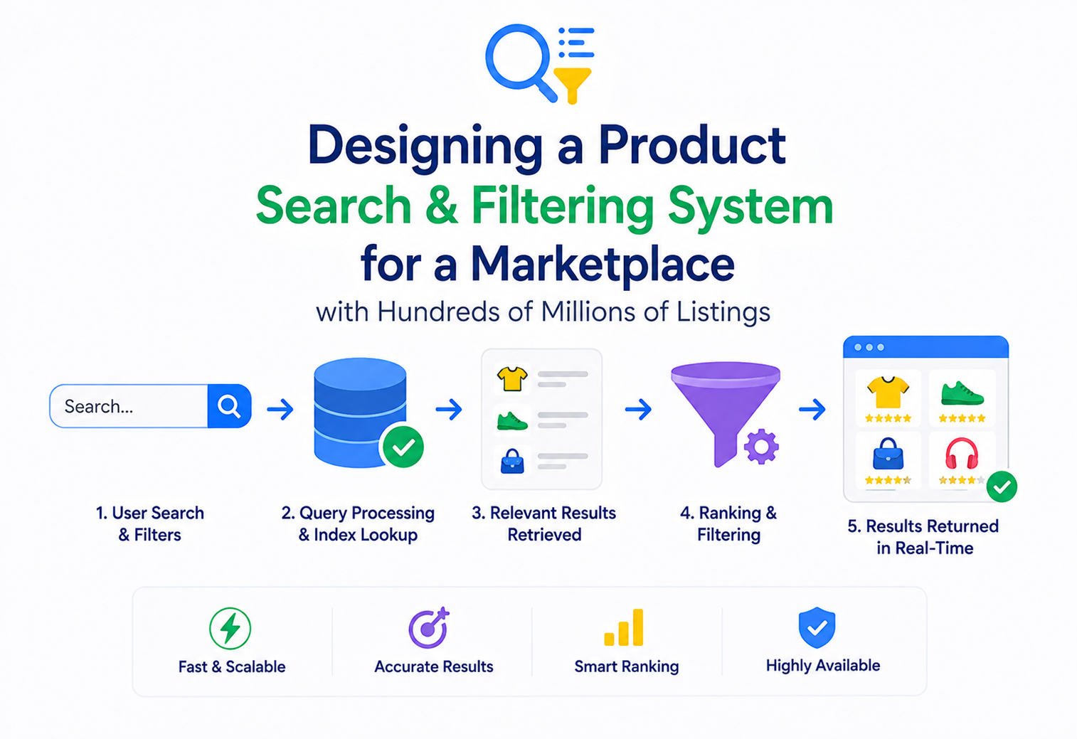
Designing a Product Search & Filtering System for a Marketplace with Hundreds of Millions of Listings
A complete, ground-up system design walkthrough: architecture, inverted-index internals, multi-attribute filtering and faceting, relevance ranking, sharding and replication, caching and load balancing, reliability, security, and the trade-offs real marketplaces make every day — from Amazon to eBay to Etsy to Uber Eats.
Introduction & History
Imagine a marketplace like the ones that sell everything from t-shirts to tractors: hundreds of millions of listings, each with dozens of attributes — brand, size, color, price, seller rating, location, delivery speed, material, and a hundred category-specific fields. Millions of buyers type a query, tap a few filters, and expect relevant results in under 200 milliseconds. That expectation — instant, relevant, filtered search over a massive and constantly changing catalog — is one of the hardest problems in distributed systems, and it sits at the center of every large e-commerce company’s engineering organization.
This tutorial builds that system from first principles. We will not assume you already know what a search index is, what a load balancer does, or why a cache exists. Every concept is explained with a real-life analogy first, then a simple example, then how it applies to production systems at companies like Amazon, Flipkart, eBay, Etsy, and Uber (for its marketplace-style listings in food and rides).
1.1 A short history of product search
In the early days of e-commerce (late 1990s), catalogs were small enough that a single relational database with a LIKE '%query%' clause could serve search. As catalogs grew into the millions, this approach collapsed — relational databases are built for exact lookups and joins, not for ranking millions of text documents by relevance.
This gave rise to a new category of software: the search engine library. Apache Lucene (1999) provided the core algorithms — inverted indexes, tokenization, relevance scoring (TF-IDF, later BM25). On top of Lucene, distributed search engines were built: Apache Solr (2004) and later Elasticsearch (2010), which added sharding, replication, and a REST API around Lucene’s core. These made it possible to search billions of documents across a cluster of machines instead of one.
In parallel, marketplaces realized that “search” is really two problems bolted together: finding relevant items for free-text queries (search) and narrowing results by exact criteria (filtering/faceting). Modern systems — the one we design here — treat these as one unified query executed against the same index, returning both ranked results and facet counts (e.g., “Color: Red (1,204), Blue (876)”) in a single round trip.

Think of a giant library with 500 million books. A relational database is like asking a librarian to read the first page of every book to check if it mentions your topic — accurate, but far too slow at this scale. A search index is like a librarian who pre-built a card catalog: for every important word, there’s a card listing every book that contains it, sorted by how relevant that book is to that word. Now the librarian only touches the cards for your search terms, not the books themselves.
Why can’t we just use a relational database with indexes for product search? — Expect you to explain that B-Tree indexes on relational databases are efficient for equality/range lookups on a few columns, but relevance ranking over free text across many fields, combined with faceted counts, requires an inverted index structure and scoring algorithms that relational engines are not built for.
1.2 How faceted search became a first-class citizen
The earliest search engines answered one question: “which documents match this text?” Marketplaces needed a second question answered in the same breath: “for every possible narrowing filter, how many results would remain?” This is what powers the familiar sidebar of checkboxes — Brand, Price Range, Color, Rating — each showing a live count next to it. Early implementations computed these counts with separate, expensive database queries per filter, which did not scale well as catalogs grew. Modern search engines solved this with aggregation frameworks built directly into the same engine that performs matching, so a single request returns both the ranked list and every facet count in one pass over the data.
This is a subtle but important evolution: search stopped being purely about relevance ranking and became a navigation tool. A user rarely knows the exact product they want; they explore through a combination of loose text (“shoes”) and progressively narrowing structured filters (brand, size, price). The system we design in this tutorial has to serve both needs from the same underlying data structure, in the same request, without sacrificing speed.
1.3 Why this matters for marketplaces specifically
A marketplace is different from a single-brand e-commerce site in one crucial way: the catalog is not curated centrally. It is contributed by potentially millions of independent sellers, each describing products in their own words, with their own attribute conventions, at their own update cadence. This means the search system must tolerate messy, inconsistent input data, normalize it into a clean schema before indexing, and still deliver consistent filtering — a shoe listed by one seller as “colour: Navy Blue” and by another as “color: navy” must both appear correctly under a single “Blue” filter option. Building this normalization layer is one of the most underestimated parts of designing marketplace search, and we will return to it when we discuss the indexing pipeline.
1.4 How to read this tutorial
We move in the order an architect would actually design this system: first understanding the problem and its constraints, then laying out the full architecture, then diving into how each piece works internally, then walking through real request flows, and finally covering the cross-cutting concerns — scalability, availability, security, and observability — that separate a toy implementation from a production-grade one serving hundreds of millions of listings. Every new term is explained in plain language before it is used technically, so no prior background in search engines or distributed systems is assumed.
Problem & Motivation
2.1 What we’re actually building
We are designing a system that lets a user type something like “waterproof running shoes size 9 under ₹3000” or select structured filters — Category: Shoes, Brand: Nike/Puma, Price: ₹1000–3000, Size: 9, Rating: 4★+, Delivery: 2-day — and receive a ranked, paginated list of matching products from a catalog of 300–800 million listings, in under 200 ms at the 95th percentile, while the catalog itself is being updated (new listings, price changes, stock changes) tens of thousands of times per second.
2.2 Core requirements
Functional requirements
- Free-text search with typo tolerance and relevance ranking
- Multi-attribute structured filtering (brand, price, size, color, rating, location, etc.)
- Faceted counts — how many results exist per filter value
- Sorting: relevance, price, rating, newest, popularity
- Pagination / infinite scroll over large result sets
- Autocomplete and query suggestions
- Personalized ranking (optional, higher-tier requirement)
- Near-real-time updates: new listings visible in seconds, price/stock updates visible almost instantly
Non-functional requirements
- p95 query latency under ~200 ms, p99 under ~500 ms
- Availability of 99.95%+ (search is revenue-critical)
- Horizontal scalability to hundreds of millions of documents and tens of thousands of queries per second (QPS)
- Eventual consistency acceptable for catalog updates (a few seconds of lag is fine); strong consistency needed for price/stock at checkout time (handled by a separate service, not search)
- Cost-efficiency at massive scale — indexing and querying hundreds of millions of documents is expensive if not engineered carefully
2.3 Who uses this system, and how that shapes design
It helps to name the distinct consumers of this system explicitly, because each pulls the design in a slightly different direction. End-user buyers browsing on web and mobile apps care most about latency and relevance quality, and are the primary driver of the sub-200-millisecond target. Internal merchandising and marketing teams need to run promotional campaigns that boost certain listings temporarily, requiring the ranking layer to support business-rule overrides without a code deployment. Partner and affiliate integrations consuming the search API programmatically need stable, versioned contracts and predictable rate limits, since they are not tolerant of the kind of breaking change a buyer-facing app team might absorb through a coordinated release. Designing for all three audiences from the start avoids costly retrofitting later.
2.4 Why this is hard
- Scale of data: Hundreds of millions of listings, each with 30–100+ attributes, means the index itself can be tens of terabytes.
- Write volume: Sellers update prices, stock, and descriptions constantly. The index must stay fresh without blocking reads.
- Combinatorial filters: A user can combine any subset of dozens of filters. Pre-computing every combination is impossible; the system must compute intersections on the fly, fast.
- Relevance vs. business logic: Pure text relevance is not enough — sponsored listings, in-stock preference, seller quality, and delivery speed all influence ranking.
- Long-tail queries: Millions of distinct queries per day, many rare, so caching alone cannot solve latency.
“We’ll just add more filters to our SQL WHERE clause and add indexes.” This works up to a few million rows with one or two filters. Once you need to combine 5–10 filters with full-text relevance ranking and facet counts across hundreds of millions of rows, relational query planners degrade sharply, and you need an inverted-index search engine purpose-built for this.
2.5 Estimating scale: back-of-the-envelope numbers
It helps to ground the design in concrete numbers before drawing any boxes. Suppose the marketplace has 500 million active listings, each averaging 2 KB of searchable data (title, description, attributes) once normalized. That is roughly 1 TB of raw searchable content before any index overhead — and inverted indexes typically add 60–120% overhead on top of raw text for term dictionaries, postings lists, and doc values, so the working index size may reach 1.5–2.5 TB. At peak, assume 50,000 queries per second (QPS) globally across all regions, each query needing to scan candidate documents, apply 3–6 filters on average, and return within 200 milliseconds. A single machine, even a powerful one, cannot hold this data in memory or serve this throughput — which is precisely why the rest of this tutorial is built around horizontal partitioning (sharding) and parallel query execution.
2.6 Read-heavy, write-frequent, not write-heavy
It is worth being precise about the write pattern. A marketplace search system is read-heavy in the sense that reads (queries) vastly outnumber writes (catalog changes) — often by a factor of 100:1 or more. But it is also write-frequent: with millions of sellers, thousands of price and stock changes occur every second in aggregate, even though any single product changes rarely. The architecture must therefore optimize primarily for read latency and throughput, while still processing a continuous, moderate stream of writes without ever falling far behind or blocking reads. This asymmetry — optimize hard for reads, keep writes flowing steadily in the background — is the central design tension of the whole system.
2.7 The filter combinatorics problem in detail
Consider a single category like “Running Shoes” with these facet dimensions: Brand (40 values), Size (15 values), Color (12 values), Price bucket (8 ranges), Rating (5 tiers), and Delivery speed (3 tiers). The number of possible filter combinations a user could construct is the product of these — into the millions — even before free-text query terms are added. Pre-computing results for every combination (a common first instinct) is completely infeasible. The only workable approach is to compute the intersection of filters at query time, using data structures fast enough that this computation, done fresh every time, still completes in milliseconds. This is exactly what an inverted index with filter-context bitsets is built for, and it is why we will spend significant time on that data structure in the next section.
Architecture & Components
Before the diagram, let’s define every component in plain language, because the diagram will name each one explicitly.
- Client: Web app, mobile app, or partner API consumer sending a search request.
- CDN (Content Delivery Network): Caches static assets (images, JS/CSS) and, in some designs, caches fully-rendered popular search result pages close to the user.
- Load Balancer (L4/L7): Distributes incoming traffic across many identical servers so no single machine is overwhelmed, and reroutes traffic away from unhealthy servers.
- API Gateway: The single front door for all client requests — handles authentication, rate limiting, request routing to the right backend service, and request/response transformation.
- Search Orchestrator Service: Parses the incoming query and filters, decides which downstream services to call, merges their responses, and applies business-logic ranking.
- Query Understanding Service: Spell correction, synonym expansion, query classification (is this a brand search? a category search?), and NLP-based intent detection.
- Search Index Cluster (Elasticsearch/Solr/OpenSearch): A distributed, sharded, replicated inverted index that executes the actual full-text search plus structured filter matching and returns ranked document IDs with facet counts.
- Ranking / Relevance Service: Applies machine-learning ranking models (Learning-to-Rank) on top of the base relevance score — factoring in click-through rate, conversion rate, personalization, and sponsored placements.
- Filter/Facet Service: Computes and formats the available filter options and counts alongside results.
- Cache Layer (Redis/Memcached): Stores results for hot queries, autocomplete suggestions, and frequently accessed facet counts.
- Product Catalog Database (sharded, e.g., MySQL/Cassandra/DynamoDB): The source-of-truth store for full product data (the index stores a searchable subset).
- Change Data Capture (CDC) + Message Queue (Kafka): Streams every create/update/delete on the catalog to the indexing pipeline in near real time.
- Indexing Pipeline / Index Builder Service: Consumes catalog change events, transforms them into index documents, and writes them into the search index cluster.
- Inventory & Pricing Service: Owns real-time stock and price truth; search index holds a near-real-time copy for filtering, but checkout always re-validates against this service.
- Autocomplete Service: A separate, latency-optimized index (often a prefix trie or a lightweight Elasticsearch index) for instant query suggestions.
- Personalization Service: Supplies user embeddings / preference signals used by the Ranking Service.
- Analytics & Logging Pipeline: Captures every query, click, and purchase for offline model training and business reporting.
- Monitoring & Alerting Stack: Tracks latency, error rate, index freshness, and cluster health.
Web Mobile Partner API”] CDN[“CDN
Static and Edge Cache”] LB[“Load Balancer
L7 NGINX or ALB”] GW[“API Gateway
AuthN Rate Limit Routing”] ORCH[“Search Orchestrator
Query Fan out and Response Merge”] QU[“Query Understanding
Spell check Synonyms Intent”] CACHE[“Cache Layer
Redis Hot Queries and Facets”] IDX[“Search Index Cluster
Elasticsearch Sharded Replicated”] RANK[“Ranking Service
Learning to Rank and Personalization”] FACET[“Filter Facet Service
Aggregation Formatting”] AC[“Autocomplete Service
Prefix Index”] PERS[“Personalization Service
User Embeddings”] CAT[“Product Catalog DB
Sharded MySQL or DynamoDB”] INV[“Inventory and Pricing Service
Source of Truth”] CDC[“CDC and Kafka
Change Stream”] IDXP[“Indexing Pipeline
Index Builder Workers”] LOG[“Analytics and Logging Pipeline”] MON[“Monitoring and Alerting
Metrics Dashboards”] Client –> CDN –> LB –> GW –> ORCH ORCH –> QU ORCH –> CACHE CACHE -.->|”cache miss”| IDX ORCH –> IDX IDX –> RANK IDX –> FACET RANK –> PERS ORCH –> AC ORCH –> LOG RANK –>|”ranked results”| ORCH FACET –>|”facet counts”| ORCH ORCH –>|”response”| GW CAT –> CDC –> IDXP –> IDX INV -.->|”price stock stream”| CDC IDX -.->|”health metrics”| MON ORCH -.->|”latency error metrics”| MON
Why separate the “Search Orchestrator” from the “Search Index Cluster”? — Because the index cluster should only do what it’s best at (matching and scoring documents), while orchestration, business-rule ranking, personalization, and calling multiple downstream services is application logic that changes often and shouldn’t live inside the search engine itself. This separation also lets you scale, deploy, and version each independently.
3.1 Why an API Gateway and Load Balancer are non-negotiable at this scale
At hundreds of millions of listings and potentially tens of thousands of queries per second, a single server can never handle the load — you need a fleet of stateless orchestrator instances behind a load balancer, which spreads requests evenly and removes unhealthy instances from rotation automatically (via health checks). The API gateway sits one layer above that fleet as the single, controlled entry point: it enforces authentication tokens, applies per-client rate limits (so one abusive script can’t degrade search for everyone), and can route different request types — search, autocomplete, filters-only — to different backend clusters.
3.2 Walking through every box again, with its job description
It helps to think of each component as an employee with one clear job, rather than a vague technical label. Below, each component from Figure 3.1 is described the way you would describe a person’s role on a team.
Load Balancer
The receptionist at the front door. Its only job is to look at incoming traffic and hand each request to a healthy, available orchestrator instance, in a way that spreads load evenly and instantly stops sending traffic to any instance that stops responding to health checks.
API Gateway
The security desk just past the receptionist. Checks identification (authentication), enforces visitor limits (rate limiting), and directs each visitor to the correct department (routing to search, autocomplete, or product-detail services) — all before any real work begins.
Search Orchestrator
The project manager. Does not do any of the specialized work itself, but knows exactly which specialists to call (query understanding, the index cluster, the ranking service), in what order, and how to assemble their outputs into one coherent answer.
Query Understanding Service
The translator. Takes what the user actually typed — often messy, misspelled, or ambiguous — and turns it into a clean, structured request the rest of the system can act on confidently.
Search Index Cluster
The card-catalog room, staffed by many librarians (shards) working in parallel. This is where the actual matching and base relevance scoring happens, at massive scale.
Ranking Service
The merchandising expert. Takes the librarians’ raw matches and re-orders them based on business goals — what tends to convert, what the user personally prefers, what sellers have paid to promote — layered on top of pure text relevance.
Indexing Pipeline
The stock room team, working continuously in the background to keep the card catalog room’s cards up to date as new inventory arrives and old inventory sells out, without ever interrupting the librarians serving customers.
Cache Layer
The frequently-asked-questions binder at the front desk. For the questions asked over and over (popular searches), the answer is already written down, so nobody needs to walk back to the card-catalog room at all.
3.3 Why the design separates “search” from “product detail” and “checkout” services
A common early-design mistake is to imagine one monolithic “Product Service” that handles searching, viewing detail pages, and purchasing. In a marketplace at this scale, these three have wildly different traffic patterns and consistency requirements: search is read-heavy and can tolerate a few seconds of staleness; a product detail page needs a mix of near-real-time price/stock and richer content; checkout needs strict, immediate consistency on price and inventory to avoid overselling. Splitting these into distinct services — each with the freshness and consistency guarantees it actually needs — is what allows the search path specifically to be aggressively optimized for speed without being held back by checkout’s stricter requirements.
Internal Working
4.1 The inverted index — the core data structure
An inverted index maps each term to the list of documents (products) that contain it, rather than mapping each document to its terms (a “forward index”). This inversion is what makes full-text search fast.
The index at the back of a textbook. Instead of reading every page to find “photosynthesis,” you look up the word once and get a list of page numbers. An inverted index does exactly this, but for every word across hundreds of millions of documents, and it also stores how relevant each page is to that word.
Beginner example
Three tiny “products”: Doc1 = “red running shoes”, Doc2 = “blue running shorts”, Doc3 = “red winter jacket”. The inverted index looks like:
"red"     -> [Doc1, Doc3]
"running" -> [Doc1, Doc2]
"shoes"   -> [Doc1]
"blue"    -> [Doc2]
"shorts"  -> [Doc2]
"winter"  -> [Doc3]
"jacket"  -> [Doc3]
A search for “red running” intersects the postings lists for “red” and “running” → only Doc1 matches both, so it ranks highest.
Production example
Elasticsearch stores this structure per shard using Lucene segments. Each field (title, description, brand, category) gets its own inverted index, plus separate structures — doc values — for fields you sort or aggregate on (price, rating), because inverted indexes are optimized for “find documents containing X,” while doc values are optimized for “get the value of field X for document Y,” which is what sorting and faceting need.

4.2 Structured filtering on top of text search
Filters like brand=Nike AND price BETWEEN 1000 AND 3000 AND size=9 are not full-text queries — they are exact/range matches. Elasticsearch handles this with filter context: filter clauses are evaluated as fast, cacheable yes/no bitsets (does this document match or not), separately from query context, where text clauses are scored for relevance. Combining them means: first narrow the candidate set with filters (cheap, cacheable), then score the remaining candidates for text relevance (more expensive, but on a much smaller set).
{
  "query": {
    "bool": {
      "must": [
        { "match": { "title": "running shoes" } }
      ],
      "filter": [
        { "term":  { "brand": "Nike" } },
        { "range": { "price": { "gte": 1000, "lte": 3000 } } },
        { "term":  { "size": 9 } },
        { "term":  { "in_stock": true } }
      ]
    }
  },
  "aggs": {
    "brand_facet": { "terms": { "field": "brand", "size": 20 } },
    "color_facet": { "terms": { "field": "color", "size": 20 } }
  }
}
The aggs block above is what produces the facet counts — “Brand: Nike (4,213), Puma (2,987)” — in the same request that returns results, avoiding a second round trip.
4.3 Relevance scoring: BM25
Modern search engines score text relevance using BM25 (Best Matching 25), a refinement of TF-IDF. It considers: how often a term appears in a document (term frequency), how rare that term is across all documents (inverse document frequency — rare terms are more informative), and document length normalization (so a short, focused title isn’t unfairly penalized against a long description stuffed with keywords).
4.4 A minimal Java client example
Here is a simplified Java snippet showing how an orchestrator service might build and send a search request to an Elasticsearch-compatible cluster using its Java client.
public SearchResponse searchProducts(SearchRequestDto req) throws IOException {
    BoolQuery.Builder boolQuery = new BoolQuery.Builder();

    // Full-text relevance clause
    boolQuery.must(m -> m.match(t -> t
        .field("title")
        .query(req.getQueryText())
    ));

    // Structured filters: fast, cacheable, not scored
    if (req.getBrand() != null) {
        boolQuery.filter(f -> f.term(t -> t.field("brand").value(req.getBrand())));
    }
    if (req.getMinPrice() != null || req.getMaxPrice() != null) {
        boolQuery.filter(f -> f.range(r -> r
            .field("price")
            .gte(JsonData.of(req.getMinPrice()))
            .lte(JsonData.of(req.getMaxPrice()))
        ));
    }
    boolQuery.filter(f -> f.term(t -> t.field("in_stock").value(true)));

    SearchRequest esRequest = SearchRequest.of(s -> s
        .index("products")
        .query(q -> q.bool(boolQuery.build()))
        .aggregations("brand_facet", a -> a.terms(t -> t.field("brand").size(20)))
        .from(req.getPageOffset())
        .size(req.getPageSize())
        .timeout("200ms")
    );

    return esClient.search(esRequest, ProductDocument.class);
}
What’s the difference between “query context” and “filter context” in a search engine, and why does the distinction matter at scale? — Filter context answers a binary yes/no and its results are cacheable as bitsets, so repeated filter combinations (e.g., in_stock=true) are nearly free on subsequent queries. Query context computes a relevance score, which is more CPU-intensive and generally not cached the same way. Structuring queries to push exact-match conditions into filter context is a major performance lever.
4.5 Typo tolerance and fuzzy matching
Users misspell queries constantly — “runing shooes” should still find “running shoes.” Search engines handle this with edit distance (also called Levenshtein distance): the minimum number of single-character insertions, deletions, or substitutions needed to turn one word into another. “Runing” is one insertion away from “Running” (edit distance 1), so a fuzzy query configured with a maximum edit distance of 1 or 2 will still match it. This fuzziness is applied selectively — usually only on the primary text fields, and only when an exact match returns too few results — because overly aggressive fuzzy matching hurts precision (you start matching genuinely unrelated words).
4.6 Synonym expansion
Beyond typos, users use different words for the same concept: “sneakers” and “shoes,” “mobile” and “smartphone,” “sofa” and “couch.” The Query Understanding Service maintains a synonym dictionary — sometimes hand-curated, sometimes mined automatically from query logs and co-click behavior — and expands the query before it reaches the index, so a search for “sneakers” also matches products only tagged “shoes” in their title.
4.7 How autocomplete works internally
Autocomplete has a much tighter latency budget than full search — typically under 50 milliseconds, because it fires on every keystroke. It is therefore backed by a separate, purpose-built structure rather than the full product index: often a prefix trie (a tree structure where each path from the root spells out a prefix) or a lightweight, heavily cached edge-n-gram index containing only popular queries and category/brand names, not full product documents. This keeps the autocomplete dataset small enough to fit comfortably in memory across all serving nodes, which is what makes single-digit-millisecond response times possible.
Full product search is like asking a research librarian to find every relevant book on a topic. Autocomplete is like asking someone standing at a directory board with the ten most popular topics memorized — they answer instantly because they only need to know a small, curated list, not the entire library’s contents.
4.8 Multi-field weighted search
A product document has many text-bearing fields — title, brand, category, description, seller name — and a match in the title should usually count for more than a match buried in the description. Search engines support field boosting, where each field is assigned a relative weight in the relevance calculation. A typical configuration might boost title by 3x, brand by 2x, and leave description at 1x, meaning a query term appearing in the title contributes three times as much to the final relevance score as the same term appearing only in the description.
4.9 Geo-spatial filtering internally
Many marketplace filters are location-based — “delivery within 2 days,” “sellers near me,” “restaurants within 5 km.” Search engines support this through specialized geo-point and geo-shape field types, indexed using structures like geohashes or quad-trees that let the engine efficiently answer “which documents fall within this radius or bounding box” without scanning every document’s coordinates individually. This is conceptually the same inverted-index principle applied to spatial data instead of text: pre-organize the data so the answer to a common question is a fast lookup, not a brute-force scan.
4.10 Personalization signals in practice
Personalization does not usually mean showing completely different results to every user; it means subtly reordering an otherwise similar candidate set based on signals like past purchase category, brand affinity inferred from click history, and price sensitivity. These signals are computed offline (in batch, by the Personalization Service) into compact per-user embeddings or feature vectors, which are fetched quickly at query time and fed into the Ranking Service’s model, rather than being computed fresh from raw history on every single search request, which would be far too slow.
4.11 Pagination and deep result sets internally
When a query fans out across many shards, each shard computes its own locally top-ranked candidates and sends them to the coordinating node, which merges and re-sorts them globally. For shallow pages (page 1, 2, 3) this is cheap. For deep pages, every shard must compute and transmit far more candidates than will actually be shown, because the globally correct top-N requires each shard to over-fetch locally. This is the underlying reason deep offset pagination becomes expensive, and why cursor-based pagination — which remembers a position and asks for “the next N after this point” rather than “skip to position 10,000” — scales far better.
Data Flow & Lifecycle
5.1 Read path: a search request end-to-end
5.2 Write path: keeping the index fresh
Sellers and internal systems constantly change product data. The index must reflect this without ever blocking a search request.
Sharded Source of Truth”] CAT –> CDC[“Change Data Capture
Debezium or Binlog Reader”] CDC –> KQ[“Kafka
Catalog Change Topic”] KQ –> IW[“Index Builder Workers
Consumer Group Horizontally Scaled”] IW –> ENR[“Enrichment Step
Category Tagging ML Embeddings”] ENR –> BULK[“Bulk Indexing API
Batched Writes”] BULK –> IDX[“Search Index Cluster
Elasticsearch or OpenSearch”] IDX –> REPL[“Replica Shards
Read Scaling and Failover”]
This design keeps writes and reads fully decoupled: even if the indexing pipeline falls behind during a traffic spike, live search queries are unaffected because they only talk to the already-built index, not the pipeline.
5.3 Consistency model
The catalog database is the source of truth and is strongly consistent for a single item. The search index is eventually consistent — typically a few seconds to a couple of minutes behind — which is an accepted trade-off because search is a discovery tool, not a transactional one. Critical fields like stock availability and price are re-validated against the Inventory & Pricing Service at the moment of add-to-cart or checkout, never trusted purely from the search index.
How would you handle a scenario where an item goes out of stock but still appears in search results for a few seconds? — Explain the trade-off: search prioritizes availability and low latency, tolerating a small consistency lag, while the checkout flow performs a real-time authoritative check against the Inventory service before confirming an order. This is the classic “eventual consistency for discovery, strong consistency for transactions” pattern.
5.4 Handling out-of-order and duplicate events
Kafka guarantees ordering only within a single partition, not across an entire topic. If catalog changes for a given product are partitioned by product ID (a deliberate design choice mentioned earlier), all updates to that one product arrive at the Index Builder Worker in the order they happened, even though updates for different products may be processed out of relative order across the cluster — which is perfectly fine, since search relevance does not depend on cross-product ordering. Each event also carries a monotonically increasing version number or timestamp, so if a worker crashes and reprocesses a batch (Kafka’s “at-least-once” delivery can redeliver messages), the Index Builder can safely discard an older version of an update that arrives after a newer one has already been applied, rather than overwriting good data with stale data.

5.5 Cache invalidation on write
A price change or a stock-out event needs to eventually be reflected not just in the index, but also in the Redis result cache, which may be holding a now-stale cached response. Rather than trying to surgically invalidate every cache entry that might reference a changed product (impractical, since a single product can appear in thousands of different query+filter cache keys), production systems rely on short TTLs (a few seconds to low minutes) for cached search results, accepting that staleness self-heals quickly through natural expiry rather than through complex targeted invalidation logic. Critical fields like stock and price are, once again, never trusted from this cache at transaction time.
5.6 Bulk reindexing flow
Beyond the steady stream of incremental updates, marketplaces periodically need a full reindex — after a schema/mapping change, a major ranking model change requiring new precomputed features, or disaster recovery. This flow reads the entire catalog database in large batches, transforms each batch through the same enrichment logic used for incremental updates, and writes into a brand-new index (not the live one) using the search engine’s bulk API for maximum throughput. Only once the new index is fully built and validated does the system flip a read alias to point at it, guaranteeing that live search traffic never sees a half-populated index during a reindex, however long it takes.
Advantages, Disadvantages & Trade-offs
| Decision | Advantage | Disadvantage / Trade-off |
|---|---|---|
| Separate search index from catalog DB | Fast, purpose-built relevance ranking and faceting at scale | Extra infrastructure, eventual consistency, need for a sync pipeline |
| Eventual consistency for indexing | Indexing pipeline never blocks reads; simpler scaling | Small windows where stale data (e.g., stock) is shown |
| Sharding the search index | Enables horizontal scale beyond a single machine’s capacity | Query fan-out overhead; harder relevance scoring across shards (global term statistics) |
| Aggressive caching of hot queries | Drastically reduces load and latency for popular searches | Cache invalidation complexity; long-tail queries get no benefit |
| ML-based re-ranking layer | Better business outcomes (CTR, conversion) beyond raw text relevance | Added latency and operational complexity of serving ML models online |
Every architectural decision in a search system is a trade-off between freshness, relevance quality, latency, and cost. You cannot maximize all four simultaneously — the job of the system designer is to choose which one your business cares about least and dial it back deliberately.
6.1 The freshness vs. cost trade-off in depth
Pushing every catalog change into the index within milliseconds is technically possible, but it means running the indexing pipeline “hot” at all times with tightly bounded batch sizes and low-latency bulk writes, which increases infrastructure cost and puts more continuous load on the same index cluster serving read traffic. Most marketplaces instead batch updates over a short window (seconds) before writing, trading a small amount of freshness for meaningfully lower cost and reduced contention on the index cluster. The right window size is itself a tuning decision made by observing real indexing lag against business tolerance for staleness.
6.2 The relevance quality vs. latency trade-off in depth
A machine-learned ranking model that considers hundreds of features (click history, conversion rates, personalization embeddings, seller quality scores) produces noticeably better business outcomes than base text relevance alone — but it costs milliseconds per candidate scored. Since scoring every one of, say, ten thousand candidate documents with a heavy model is too slow, production systems apply a two-stage ranking approach: a cheap, fast method (base relevance, or a lightweight model) narrows millions of matches down to a few hundred candidates, and only those few hundred are scored by the expensive, high-quality model. This “retrieve cheap, rank expensive on a small set” pattern recurs throughout large-scale search and recommendation systems.
6.3 The precision vs. recall trade-off
Widening fuzzy matching and synonym expansion increases recall (fewer relevant items missed) but risks reducing precision (more irrelevant items included). A search for “apple” without any disambiguation could return both fruit and electronics, depending on category context. Marketplaces manage this trade-off through category-aware query understanding — using the user’s browsing context, past behavior, or an explicit category filter to disambiguate — rather than trying to solve ambiguity purely at the text-matching level.
Performance & Scalability
7.1 Sharding the search index
A single machine cannot hold hundreds of millions of documents with acceptable query latency, so the index is split into shards — independent, self-contained pieces of the total index — distributed across many machines. A query fans out to all relevant shards in parallel, and each shard returns its top candidates, which the orchestrator merges.
Instead of one librarian searching all 500 million books, you hire 200 librarians, each responsible for 2.5 million books. You ask your question to all 200 at once; each searches their own section in parallel and reports their best matches back to a head librarian, who merges the 200 answer lists into one final list.
Sharding strategy
Common approaches: shard by a hash of product ID (even distribution, simple), or shard by category (keeps category-scoped queries fast but risks hot shards for popular categories like “Mobiles”). Most large marketplaces use hash-based sharding with a high shard count and rely on replicas plus caching to handle hot categories, since hash-based sharding avoids the imbalance problem entirely.
7.2 Replication for read scaling
Each shard has multiple replicas. Replicas serve read (search) traffic in round-robin, multiplying query throughput, and provide failover if a primary shard’s node goes down.
7.3 Query-time optimizations
- Filter caching: Frequently used filter clauses (e.g.,
in_stock=true, common category IDs) are cached as bitsets at the shard level. - Result caching: The orchestrator caches full responses for hot query+filter combinations (e.g., “iPhone” with no filters) with a short TTL (seconds to low minutes).
- Pagination limits: Deep pagination (page 500) is expensive in distributed search; production systems cap visible pages and push users toward refining filters instead, or use
search_aftercursor-based pagination rather than offset-based. - Field selection: Only fetching the fields actually needed for the results grid (not full product descriptions) reduces network and serialization cost.
7.4 Scaling the indexing pipeline
Kafka partitions allow many Index Builder Worker instances to consume catalog changes in parallel. Partitioning by product ID ensures all updates for a given product are processed in order (avoiding a race where an older update overwrites a newer one), while still allowing horizontal scaling across many partitions.
How would you scale search from 10 million to 500 million products? — A strong answer covers: increasing shard count (with a re-index/split strategy, since shard count is hard to change after index creation in most engines), scaling out replicas for read throughput, moving from offset to cursor-based pagination, introducing tiered caching, and possibly splitting the single monolithic index into category-specific indexes with a routing layer if certain categories dominate traffic.
7.5 Choosing the right shard count
Shard count is one of the few decisions that is expensive to change after the fact in most search engines, because it is fixed at index creation time — changing it typically requires creating a new index with the new shard count and reindexing everything into it. Too few shards means each shard grows too large, hurting both query latency and the time needed to recover a failed node (since a bigger shard takes longer to copy when rebuilding a replica). Too many shards adds coordination overhead per query, since the orchestrating node must fan out to and merge results from every shard, even ones with little relevant data. A common rule of thumb is to size each shard so it comfortably fits in the available memory/disk of a single node, typically somewhere in the tens of gigabytes, and choose the total shard count accordingly, planning ahead for a reasonable growth horizon rather than the current catalog size alone.
7.6 Hot shard mitigation
Even with hash-based sharding, certain query patterns can concentrate load unevenly — for example, if a promotional campaign drives a surge of “mobile phones” category traffic, and category happens to correlate with certain hash ranges. Marketplaces mitigate this with a combination of a higher shard count than strictly necessary (giving the load balancer more granular units to spread across nodes), replica-level load balancing (round-robining reads across all replicas of a shard, not just the primary), and application-level caching that absorbs the bulk of repeat traffic for trending queries before it ever reaches the index cluster at all.
7.7 Precomputed aggregations for common facets
While most facet counts must be computed at query time because they depend on the specific filter combination applied, some coarse-grained aggregates — such as total product count per top-level category — change slowly enough and are requested often enough that they are worth precomputing and refreshing periodically (e.g., every few minutes) rather than recalculated on every request, further reducing load on the index cluster for the most common query shapes.
7.8 Autoscaling considerations
Stateless layers (API Gateway, Orchestrator, Ranking Service instances) scale horizontally in response to CPU or request-queue-depth signals within seconds. The search index cluster, being stateful, cannot scale nearly as fast — adding a node means that node must receive a copy of shard data before it can serve meaningful traffic, which can take minutes to hours depending on shard size and network bandwidth. Capacity planning for the index cluster is therefore done proactively based on projected catalog and traffic growth, with a comfortable headroom buffer, rather than relying purely on reactive autoscaling the way stateless services can.
High Availability & Reliability
8.1 Redundancy at every layer
No single component should be a single point of failure. Load balancers are deployed in active-active pairs; API gateway and orchestrator instances run across multiple availability zones; the search index cluster maintains at least one replica per shard, ideally spread across zones; Kafka topics are replicated across brokers.
8.2 Graceful degradation
When the Ranking/Personalization service is slow or down, the orchestrator should fall back to base relevance scores rather than failing the whole request — a degraded but working search result beats an error page. This is implemented with timeouts and circuit breakers around every downstream call.
8.3 Circuit breaker pattern in Java (conceptual)
public RankedResults getRankedResults(List<Product> candidates, String userId) {
    try {
        return rankingCircuitBreaker.executeSupplier(() ->
            rankingService.rank(candidates, userId)
        );
    } catch (CallNotPermittedException | TimeoutException ex) {
        // Fallback: return base relevance order without personalization
        log.warn("Ranking service degraded, falling back to base scores");
        return RankedResults.fromBaseScores(candidates);
    }
}
8.4 Disaster recovery
Search index snapshots are taken periodically (e.g., every few hours) and stored in durable object storage. Since the index can always be fully rebuilt from the catalog database plus the Kafka change log, the index cluster itself is treated as disposable/rebuildable state, not a permanent source of truth — which greatly simplifies disaster recovery.
If your entire search index cluster is lost, how do you recover? — Because the catalog DB is the source of truth and Kafka retains recent change history, you can spin up a fresh cluster and replay the full catalog (bulk re-index) plus any missed Kafka messages to rebuild the index from scratch, rather than relying solely on backups.
8.5 Health checks and automatic failover
Every layer performs its own form of health checking. The load balancer periodically pings each orchestrator instance and removes any that fail to respond within a threshold. The search index cluster runs its own internal cluster coordination (historically via a consensus mechanism, now often a dedicated cluster-manager node role) to detect a failed node and automatically promote a healthy replica shard to primary, so no single node failure ever makes a shard of data unavailable. This automatic promotion typically happens within seconds, well within the tolerance of client-side retry logic in the orchestrator.
8.6 Timeouts, retries, and idempotency
Every network call in the system — orchestrator to index cluster, orchestrator to ranking service, index builder to search index — is wrapped with an explicit timeout, because an unbounded wait on a slow dependency is far more damaging than a fast failure the caller can react to. Retries are used carefully and only for idempotent operations (safe to repeat without side effects, like a read query), never blindly applied to writes, to avoid issues like double-indexing the same catalog change. Exponential backoff with jitter is used on retries to avoid a “thundering herd” where many clients retry a struggling service at exactly the same moment, making its recovery harder.
8.7 Load shedding under extreme traffic
During extreme spikes — a major sale event, for instance — the system may receive more traffic than it can serve while maintaining target latency for everyone. Rather than letting every request degrade uniformly into slow, timing-out responses, mature systems implement load shedding: the API Gateway or Orchestrator detects it is approaching capacity and starts intentionally rejecting a small percentage of lower-priority requests (e.g., non-critical autocomplete calls) early and cheaply, protecting latency and success rate for the core search requests that matter most to revenue.
8.8 Chaos engineering and failure testing
Large marketplaces regularly and deliberately inject failures into non-production, and sometimes production, environments — killing an index node, introducing artificial network latency between services, or simulating a full availability-zone outage — to validate that the redundancy and fallback mechanisms designed on paper actually work under real conditions, rather than assuming they do because the architecture diagram looks correct.
Security
- AuthN/AuthZ at the gateway: API keys or OAuth tokens for partner APIs; session tokens for consumer apps, validated once at the API Gateway so downstream services trust a signed internal token.
- Rate limiting & abuse prevention: Per-client and per-IP rate limits at the gateway prevent scraping of the entire catalog and protect against denial-of-service via expensive queries (e.g., deep pagination or wildcard-heavy searches).
- Query sanitization: User input is never passed directly into a raw query DSL string; it is parsed into structured query objects to prevent search-engine injection attacks.
- Field-level access control: Internal-only fields (seller cost price, fraud scores) are excluded from any index or API response reachable by end users.
- Data-in-transit and at-rest encryption: TLS between all services; encrypted storage volumes for the index and catalog data, particularly where seller PII is involved.
- Seller data isolation: Multi-tenant marketplaces must ensure one seller cannot query or infer another seller’s private analytics through crafted search/facet requests.
Exposing the raw search-engine query DSL directly to client applications. This lets a malicious or buggy client submit expensive, unbounded queries (e.g., huge aggregation bucket sizes) that can degrade the whole cluster. Always mediate through the orchestrator, which validates and bounds every parameter.
9.1 Protecting against catalog scraping
A marketplace’s product catalog, pricing, and seller data are valuable competitive information, and search APIs are the most convenient path for a competitor or bot to scrape the entire catalog systematically. Beyond simple rate limiting, mature systems apply behavioral detection — flagging clients that page through results unusually fast, in unusually exhaustive patterns, or with request signatures inconsistent with a real browser or app — and can respond with CAPTCHAs, temporary throttling, or outright blocking, without impacting legitimate users.
9.2 Protecting seller and buyer privacy
Facet aggregations, if not carefully scoped, can leak information that was never meant to be exposed — for example, allowing someone to infer a specific seller’s exact inventory count or sales patterns by cleverly combining filters. Search response payloads are designed to only ever include fields explicitly meant for public buyer-facing display, with a strict allow-list rather than a block-list approach to field exposure, since a block-list is easy to forget to update when new internal fields are added to the underlying catalog schema.
9.3 Securing the indexing pipeline
The indexing pipeline itself is an internal, trusted path, but it is not exempt from security controls — Kafka topics carrying catalog change events are access-controlled so only authorized services can produce or consume from them, and the Index Builder Workers validate and sanitize incoming data even though it originates from an internal system, since a compromised or buggy upstream service should never be able to inject malformed or malicious content directly into the publicly served search index.
Monitoring, Logging & Metrics
10.1 What to monitor
| Category | Key Metrics |
|---|---|
| Latency | p50/p95/p99 query latency, per endpoint and per downstream dependency |
| Availability | Error rate, timeout rate, circuit breaker open/close events |
| Index Health | Cluster status (green/yellow/red), shard allocation, indexing lag (time from catalog change to searchable) |
| Relevance Quality | Click-through rate on top results, zero-result-query rate, conversion rate by query |
| Capacity | QPS per shard, CPU/heap usage per node, queue depth in Kafka consumers |
| Cache | Hit ratio, eviction rate, memory usage |
10.2 Distributed tracing
A single search request touches many services (gateway, orchestrator, query understanding, index, ranking, personalization). Distributed tracing (e.g., OpenTelemetry with a trace ID propagated through every hop) lets engineers see exactly where time is spent for a slow request, rather than guessing.
10.3 Zero-result and low-relevance monitoring
Beyond system health, marketplaces track business-relevant search metrics: the percentage of queries returning zero results (a discovery failure), and queries with results but no clicks (a relevance failure). These feed back into the Query Understanding and Ranking services as training signals.
How do you know your search results are actually good, not just fast? — Discuss offline relevance evaluation (labeled query-result relevance datasets, NDCG scoring), online A/B testing of ranking changes, and production signals like CTR, zero-result rate, and conversion rate, tied back to specific query segments.
10.4 Structured logging for every search request
Every search request logs a structured record — query text, applied filters, result count, top result IDs, latency breakdown per downstream call, and the eventual user action (click, add-to-cart, purchase, or abandonment) joined in asynchronously. This log is the raw material for almost everything else in the system’s feedback loop: relevance model training, A/B test analysis, business reporting on category-level demand, and debugging individual user complaints about “search isn’t finding what I want.”
10.5 Alerting philosophy
Good alerting distinguishes between symptoms and causes, and alerts primarily on symptoms that matter to users — elevated p99 latency, elevated error rate, a spike in zero-result queries — rather than every possible internal metric crossing a threshold. Alerting on every internal cause (e.g., one node’s CPU briefly spiking) leads to alert fatigue, where engineers start ignoring pages, which is far more dangerous than having fewer, well-chosen alerts tied to actual user impact.
10.6 Dashboards for different audiences
Engineering teams need low-level dashboards: per-shard latency, cache hit ratios, Kafka consumer lag. Business and product teams need a different view: search conversion rate by category, top zero-result queries this week, and the impact of a recent ranking experiment on revenue. Building both from the same underlying structured logs, rather than maintaining two separate logging pipelines, keeps the numbers consistent across engineering and business reporting.
Deployment & Cloud
11.1 Containerized, orchestrated services
Stateless services (API Gateway, Orchestrator, Query Understanding, Ranking, Autocomplete) are packaged as containers and run on an orchestration platform (Kubernetes) with horizontal pod autoscaling based on CPU and request-queue metrics. Stateful components (search index cluster, Kafka, catalog database) run as managed services or dedicated StatefulSets with careful capacity planning, since scaling stateful systems is riskier and slower than scaling stateless ones.
11.2 Multi-region considerations
For marketplaces operating across countries, search infrastructure is typically deployed per-region (or per major geography) to keep latency low and comply with data residency regulations, with the catalog database replicated regionally and the indexing pipeline running independently per region.
11.3 Blue-green and canary deployments
Ranking model updates and orchestrator releases are rolled out via canary deployment — a small percentage of traffic hits the new version first, monitored closely for latency and relevance regressions, before a full rollout. This is critical because a bad ranking model can silently hurt conversion without causing visible errors.
Why deploy search index nodes differently from the stateless application services? — Because index nodes hold large amounts of local disk-backed data (shards) and rebalancing/adding nodes is expensive and slow (data must be copied), unlike stateless services that can be scaled up or down instantly. This means capacity planning for the index cluster must be proactive, not purely reactive autoscaling.
11.4 Infrastructure as code
Every environment — the index cluster’s node configuration, Kafka topic partition counts, autoscaling policies, alerting thresholds — is defined declaratively in version-controlled configuration rather than manually configured through a console. This means a new region or a disaster-recovery environment can be stood up predictably and repeatably, and any configuration drift between environments becomes visible as a diff rather than a mystery discovered during an incident.
11.5 Cost optimization at scale
At hundreds of millions of documents, the search index cluster is one of the largest line items in infrastructure cost. Common cost levers include: tiering hardware, keeping recently updated and heavily queried “hot” data on fast local SSD-backed nodes while moving older, rarely filtered historical or archival data to cheaper storage tiers; right-sizing replica counts per shard based on actual read traffic rather than a flat default; and using compressed field storage (excluding fields from the index that are never searched or filtered on, and only ever displayed from the catalog database directly on a product detail page).

11.6 Environment parity
Staging and testing environments run a scaled-down but structurally identical version of the production topology — same number of logical layers, same sharding strategy at a smaller shard count — so that performance and correctness issues surface before a release reaches production, rather than only appearing once real scale is applied.
Databases, Caching & Load Balancing
12.1 Product catalog database
The catalog database is typically a horizontally sharded relational store (e.g., MySQL with application-level sharding) or a distributed NoSQL store (e.g., DynamoDB, Cassandra) keyed by product ID, optimized for high-throughput writes and simple key-based reads (fetching one product’s full detail page), not for complex ad-hoc search.
12.2 Caching layers
| Layer | Purpose | Typical TTL |
|---|---|---|
| CDN edge cache | Popular category/landing page results | Minutes |
| Redis result cache | Hot query+filter combinations | Seconds to a few minutes |
| Autocomplete cache | Prefix suggestions for common prefixes | Hours, refreshed periodically |
| Filter bitset cache (index-internal) | Frequently used exact-match filters | Managed internally by the search engine |
12.3 Multi-tier caching strategy in practice
Rather than relying on a single cache layer, production marketplace search systems typically layer caching at three levels working together. At the outermost edge, the CDN caches fully rendered responses for anonymous, non-personalized landing and category pages, since these are identical for every visitor and change infrequently. One layer in, the Redis result cache stores personalization-agnostic base result sets keyed by the normalized query and filter combination, serving as the workhorse cache absorbing the majority of repeat traffic. Innermost, the search engine’s own internal filter-bitset and query caches speed up even cache-missed requests by reusing previously computed filter intersections. Each layer catches a different slice of repeat traffic, and together they mean only a small fraction of requests ever need a full, uncached pass through the index cluster.
12.4 Cache key design
Designing the cache key correctly is subtle: it must include every input that affects the response (query text, all applied filters, sort order, page number, locale/currency) while excluding inputs that do not (a request trace ID, for instance), or the cache will either serve incorrect stale results for a slightly different request, or fail to get any cache hits at all because keys are needlessly unique. A common approach is to canonicalize the filter set (sorting filter keys alphabetically, normalizing value casing) before hashing it into the cache key, so that logically identical requests arriving with parameters in a different order still produce the same cache key and benefit from the same cached entry.
12.5 Load balancing strategy
Layer 7 (application-aware) load balancing is preferred over simple Layer 4, because it can route based on request path (e.g., /search vs /autocomplete vs /product/{id}) to different backend pools, apply weighted routing for canary releases, and terminate TLS centrally.
A Layer 4 load balancer is like a receptionist who only looks at which door you came through and sends you to any available room. A Layer 7 load balancer is like a receptionist who reads your request form and sends “search” requests to the search team’s floor and “checkout” requests to the payments floor — smarter routing based on content, not just connection.
12.6 Why the catalog database is sharded independently from the search index
It is worth being explicit that the catalog database’s sharding strategy and the search index’s sharding strategy are entirely independent decisions, optimized for different access patterns. The catalog database is typically sharded by product ID or seller ID because its dominant access pattern is “fetch this one product” or “fetch all products for this seller,” both of which benefit from routing directly to the shard owning that key. The search index is sharded (as discussed earlier) primarily for even distribution of a very different access pattern — broad queries that must touch data across the entire catalog. Conflating these two sharding strategies, a mistake sometimes made by teams new to this architecture, leads to a system optimized for neither workload well.
12.7 Read replicas for the catalog database
Beyond the search index’s own replicas, the catalog database itself typically runs read replicas to serve the Indexing Pipeline’s bulk-read workloads (during full reindexes) without competing for capacity with the primary database instances serving live seller-facing writes (price updates, new listings) and buyer-facing product detail page reads.
12.8 Choosing between Elasticsearch, Solr, and OpenSearch
All three are built on Apache Lucene and share the same core inverted-index concepts described in this tutorial, but differ in ecosystem, licensing, and operational tooling. Elasticsearch offers a mature managed-service ecosystem and rich aggregation APIs; Apache Solr has a longer history in some enterprise search deployments and strong support for complex faceting configurations; OpenSearch is a community-driven, permissively licensed fork of Elasticsearch that gained adoption after Elasticsearch’s licensing changes. For a system design discussion, the important point is that the architectural patterns in this tutorial — filter context, sharding, replication, aggregations — apply essentially identically across all three, since they share the same Lucene foundation.
12.9 Session and rate-limit state
The API Gateway and Orchestrator layers are designed to be stateless with respect to application logic, but rate-limiting and session-validation state must still be tracked somewhere shared across all gateway instances — typically in a fast, distributed cache like Redis, using counters with a sliding or fixed time window, so that a client’s rate limit is enforced consistently no matter which gateway instance happens to handle a particular request.
APIs & Microservices
13.1 Service boundaries
Each component from the architecture diagram is typically its own independently deployable microservice, communicating over synchronous REST/gRPC for request-time calls (orchestrator → index cluster, orchestrator → ranking service) and asynchronous events (Kafka) for the indexing pipeline.
13.2 Sample REST API contract
GET /api/v1/search?q=running%20shoes&brand=Nike&price_min=1000&price_max=3000&size=9&sort=relevance&page=1&page_size=24

Response:
{
  "results": [
    {
      "id": "PROD-88213",
      "title": "Nike Revolution 6 Running Shoes",
      "price": 2499,
      "rating": 4.3,
      "in_stock": true,
      "score": 12.87
    }
  ],
  "facets": {
    "brand": [ {"value": "Nike", "count": 4213}, {"value": "Puma", "count": 2987} ],
    "color": [ {"value": "Black", "count": 3120}, {"value": "White", "count": 1876} ]
  },
  "pagination": { "page": 1, "page_size": 24, "total_estimated": 6412 },
  "took_ms": 87
}
13.3 gRPC for internal service-to-service calls
While the public API is REST/JSON for broad client compatibility, internal calls (orchestrator to ranking service, orchestrator to personalization service) often use gRPC for lower latency and strongly typed contracts, since these calls happen multiple times per single user request and shave off meaningful milliseconds at scale.
Would you expose the search index cluster’s native API directly to your mobile app? — No — always mediate through an orchestrator/API layer, because it lets you change the underlying search engine, add caching, apply business rules, and protect against expensive or malicious queries without ever touching client applications.
13.4 Versioning the search API
As ranking logic, response fields, and facet structures evolve, the public search API is versioned explicitly (as seen in the /api/v1/search path above) so that older client app versions still in use by users who have not updated their app continue to receive a response shape they understand, while new clients can opt into a newer version with additional fields or behavior. Breaking changes are never pushed silently into an existing version.
13.5 Backward and forward compatibility in event schemas
The Kafka catalog-change event schema follows the same discipline: new optional fields can be added freely, but existing fields are never removed or repurposed, and consumers (the Index Builder Workers) are written to safely ignore fields they do not yet understand. This allows the catalog service team and the search team to deploy independently, on their own schedules, without a fragile coordinated release.
13.6 Service ownership and team boundaries
In a large engineering organization, each of the microservices in this architecture is typically owned by a distinct team: a Catalog team owns the product database and seller-facing APIs; a Search Platform team owns the index cluster, orchestrator, and query understanding; a Relevance/Ranking team owns the ranking models and personalization signals; a Platform Infrastructure team owns the shared Kafka, monitoring, and deployment tooling. Clear API contracts between these services are what allow dozens of engineers across multiple teams to work on this system concurrently without constantly blocking on each other.
13.7 Internal API example: Ranking Service gRPC contract
public interface RankingServiceClient {
    RankResponse rank(RankRequest request);
}

public class RankRequest {
    private String userId;
    private List<CandidateDocument> candidates; // typically a few hundred, not millions
    private String queryText;
    private Map<String, String> appliedFilters;
    private long requestTimestamp;
}

public class RankResponse {
    private List<ScoredDocument> rankedCandidates;
    private String modelVersion; // for experiment tracking and rollback
}
Notice that this internal contract only ever receives a small, already-narrowed candidate set (from the two-stage retrieve-then-rank pattern discussed earlier), never the full result set from the index — reinforcing, at the API boundary itself, the architectural principle that expensive ranking only ever runs on a bounded number of candidates.
Design Patterns & Anti-patterns
14.1 Patterns used
CQRS
Command Query Responsibility Segregation: writes go to the catalog DB; reads go to the search index — two different, independently optimized models for the same data.
Event Sourcing / CDC
The Kafka change stream acts as an ordered log of everything that happened to the catalog, which the index (and other consumers, like analytics) can replay.
Circuit Breaker
Protects the orchestrator from cascading failures when a downstream service (ranking, personalization) is unhealthy.
Bulkhead
Separate thread pools / connection pools per downstream dependency so a slow ranking service can’t exhaust resources needed for basic search.
Cache-Aside
The orchestrator checks the cache first, and on a miss, queries the index and populates the cache — a classic and simple caching pattern.
Two-Stage Ranking
A cheap, fast retrieval narrows millions of matches down to a small candidate set; only that small set is scored by the expensive, high-quality ranking model.
14.2 Anti-patterns to avoid
- Using the search index as the system of record. It should always be rebuildable from the catalog DB; treating it as primary storage risks permanent data loss on corruption.
- Deep offset-based pagination. Requesting page 10,000 forces the engine to compute and discard everything before it — replace with cursor/search-after based pagination.
- One giant index for everything. Mixing wildly different document shapes (products, sellers, reviews) in a single index complicates mapping management and mapping explosion; use separate indexes per entity type.
- Synchronous indexing on the write path. Making a product-save API call wait for the search index to update couples an unrelated system’s latency and availability to a core write path — always index asynchronously.
- No query timeout. A single expensive query without a timeout can consume disproportionate cluster resources and degrade every other concurrent query.
Treating relevance tuning as a “set it once” activity. Search relevance requires continuous tuning as catalog composition, user behavior, and business priorities shift — mature teams run relevance as an ongoing experimentation program, not a one-time configuration.
14.3 The strangler fig pattern for migrations
When a marketplace migrates from an older search stack to a new one — for example, moving off a legacy self-hosted setup onto a modern managed cluster — it is rarely done as a single risky cutover. Instead, the strangler fig pattern routes a small, increasing percentage of traffic to the new system while the old one keeps serving the rest, with both systems fed by the same indexing pipeline, until confidence in the new system’s correctness and performance is high enough to fully retire the old one. This pattern is what allows a live, revenue-critical system to be re-architected without a risky big-bang cutover.
14.4 The Saga pattern’s relevance here
While search itself is a read path and does not typically need distributed transactions, the broader catalog-update workflow — a seller updating a listing, which must propagate to the catalog database, the search index, and possibly a recommendations service — resembles a saga: a sequence of local updates across services, coordinated through events rather than a single distributed transaction, with each service responsible for eventually converging rather than requiring instantaneous cross-service atomicity.
14.5 Anti-pattern: tight coupling between ranking logic and index schema
A subtle anti-pattern is embedding business ranking logic (such as boosting sponsored listings) directly as index-time scoring boosts baked into the document mapping, rather than as a separate, versionable layer applied at query or ranking-service time. Baking business logic into the index schema means changing a ranking rule requires a full reindex, whereas keeping it in the Ranking Service means a ranking change can be deployed and rolled back independently, in minutes, without touching the index at all.
Best Practices & Common Mistakes
15.1 Best practices
- Push exact-match conditions into filter context, not query context, for performance and cacheability.
- Keep the index schema (mapping) versioned and use index aliases so you can rebuild a new index and switch traffic atomically with zero downtime.
- Set conservative query timeouts and enforce maximum page size / aggregation bucket limits at the API layer.
- Separate the autocomplete index from the main product index — they have very different latency and freshness requirements.
- Continuously monitor indexing lag as a first-class SLO, not an afterthought.
- Design the catalog change schema to be additive and backward-compatible so index builder workers can be deployed independently of catalog schema changes.
- Load test with realistic filter-combination distributions, not just simple text queries — filter-heavy queries stress a different part of the system.
15.2 Common mistakes
- Under-provisioning shard count early and being forced into a painful full re-index later to change it.
- Ignoring “zero-result” queries as a metric, missing major discovery gaps in the catalog or query understanding logic.
- Coupling ranking business logic tightly inside the search engine’s native scripting, making it hard to test, version, and roll back independently.
- Not isolating noisy-neighbor tenants (large sellers with huge catalogs) whose bulk updates can overwhelm the indexing pipeline for everyone else.
How would you support atomic reindexing with zero downtime after a mapping/schema change? — Explain the index-alias pattern: build a brand-new index with the new mapping, backfill it fully from the catalog, then atomically flip a read alias from the old index to the new one, so clients never see a broken or half-migrated index.
15.3 Testing search quality, not just search correctness
Unit and integration tests can confirm that a query returns syntactically correct results, but they cannot confirm the results are actually good. Mature teams maintain a curated set of representative query-result relevance judgments (often gathered through human evaluation or inferred from strong click/conversion signals) and run automated relevance regression checks — computing metrics like NDCG (Normalized Discounted Cumulative Gain) — against this judged set on every significant ranking or query-understanding change, catching relevance regressions before they ever reach real users.
15.4 Runbooks for common incidents
Because search sits directly on the revenue path, teams maintain runbooks for the most common failure modes — an index cluster turning yellow or red, indexing lag spiking beyond a threshold, a sudden drop in query success rate — with clear, pre-agreed steps for on-call engineers, rather than improvising under pressure during an actual incident.
15.5 Progressive rollout of new attributes and filters
Adding a brand-new filterable attribute across hundreds of millions of existing listings (for example, introducing a “Sustainability Rating” filter) requires backfilling that attribute for the entire existing catalog, which can take significant time. Best practice is to roll this out progressively — starting with new listings, backfilling older ones in batches during low-traffic periods — and only surface the new filter in the user interface once backfill coverage is high enough that the filter is actually useful, rather than exposing a filter that silently excludes most of the catalog on day one.
Real-World / Industry Examples
Amazon
Uses a proprietary distributed search platform (historically built on principles similar to A9 search) that combines text relevance with heavy business-signal ranking — sales velocity, Prime eligibility, and sponsored placement — layered on top of base relevance, illustrating how commercial ranking diverges from pure information retrieval.
eBay
Operates one of the largest Apache Lucene/Solr-derived deployments in e-commerce, handling structured, highly variable item attributes (a defining eBay challenge, since sellers define semi-custom item specifics) alongside free-text search.
Uber Eats / Food Marketplaces
Combine geo-spatial filtering (restaurants within delivery radius) with menu-item text search and real-time availability — an example of filters that are inherently time- and location-sensitive, requiring tight integration between search and live operational data.
Etsy
Publicly documented moving from a legacy search stack to Elasticsearch, emphasizing machine-learned ranking to balance relevance with marketplace health goals like seller diversity and discovery of smaller sellers, not just raw popularity.
Across all of these, the recurring architectural theme is the same one this tutorial builds: a fast, purpose-built search index decoupled from the transactional catalog database, kept fresh via an asynchronous pipeline, fronted by an orchestration layer that blends relevance with business logic.
16.1 What varies across these companies
Despite the shared architectural skeleton, real implementations diverge based on business priorities. A marketplace with highly standardized products (electronics, books) can rely heavily on structured attribute filtering with relatively light text-relevance needs, since a query like “iPhone 15” has an almost unambiguous correct answer. A marketplace with highly variable, seller-described items (handmade goods, used items, local classifieds) leans much more heavily on text relevance, synonym handling, and tolerant fuzzy matching, since sellers rarely describe similar items identically. Recognizing which end of this spectrum a given marketplace sits closer to is one of the first judgment calls a system designer makes, because it shapes how much investment goes into query understanding versus structured filtering infrastructure.
16.2 Lessons learned across the industry
- Relevance and business ranking are never “finished” — every company referenced here treats it as a continuously iterated system backed by experimentation, not a static configuration set once at launch.
- Facet and filter design is as much a product/UX discipline as an engineering one — which filters to surface, and in what order, meaningfully affects discovery and conversion, not just the underlying query performance.
- Geo-aware and time-aware filtering (delivery estimates, local availability) has become table stakes for marketplaces with physical fulfillment, requiring tight integration between the search layer and real-time logistics/inventory systems, well beyond a static catalog index.
FAQ, Summary & Key Takeaways
17.1 Frequently asked questions
Why not just use the catalog database with strong indexes for filters?
Relational indexes work well for a small number of equality/range conditions on a modest dataset. Once you need free-text relevance ranking, faceted aggregation, and arbitrary combinations of many filters across hundreds of millions of rows with sub-200ms latency, an inverted-index search engine is purpose-built for this and a relational engine is not.
How fresh does the index need to be?
Most marketplaces target seconds-to-low-minutes freshness for general catalog data, with special low-latency paths (sometimes near-synchronous) for critical fields like stock status, and a hard rule that checkout always re-validates price/stock against the authoritative Inventory service rather than trusting the index.
How do you handle typos and synonyms?
The Query Understanding Service applies fuzzy matching (edit-distance based) for typo tolerance and a synonym dictionary (e.g., “sneakers” ↔ “shoes”) before the query reaches the index, and the index itself can also apply fuzziness at the field level for additional tolerance.
What happens when a filter combination has zero results?
The Filter/Facet Service can suggest the “nearest” relaxation — e.g., widen the price range or drop the least-selected filter — computed by re-running facet aggregation without one filter at a time to find which single relaxation restores results.
How is this different from a general-purpose web search engine like Google?
A general web search engine ranks a heterogeneous, largely unstructured web of pages using signals like link authority and content quality, with far less rigid structured filtering. Marketplace search, by contrast, operates over a homogeneous set of structured entities (products) with well-defined attributes, and faceted filtering is a first-class, heavily used feature rather than a secondary capability — which is why aggregation performance and filter-context caching receive so much architectural attention in this tutorial.
Do all hundreds of millions of listings need to be in a single index?
Not necessarily. Large marketplaces sometimes split the index by top-level category or by region when query patterns rarely cross those boundaries, which can reduce the effective document count any single query needs to consider and simplify capacity planning per vertical. The trade-off is added routing complexity in the orchestrator, which must know which index (or indexes) to query for a given request, and more complex cross-category search scenarios.
How do sponsored or promoted listings fit into this architecture?
Sponsored listings are typically handled as an additional signal blended in at the Ranking Service stage, not as a separate search path — the base index returns organically relevant candidates, and the ranking layer interleaves or boosts sponsored candidates according to business rules and auction mechanics, while still respecting relevance thresholds so that irrelevant sponsored items are not forced in front of users, which would damage trust and long-term engagement.
What is the single biggest scaling bottleneck teams underestimate?
Most teams correctly anticipate that the search index itself needs to scale, but underestimate how quickly the indexing pipeline and catalog change volume grow as seller count increases, and end up needing to re-architect the Kafka partitioning and Index Builder Worker scaling strategy under pressure, later than would have been ideal. Planning the write path’s scalability with the same rigor as the read path from the start avoids this.
17.2 Summary
Designing product search and filtering at marketplace scale means treating search as a dedicated read-optimized system, fully decoupled from the transactional catalog database, fed by an asynchronous indexing pipeline, sharded and replicated for horizontal scale, fronted by a load balancer and API gateway, and orchestrated by a service layer that blends raw relevance with business-driven ranking — all wrapped in caching, monitoring, and graceful-degradation patterns that keep the system fast and available even when individual components fail.
- Inverted indexes, not relational tables, are the right data structure for large-scale relevance-ranked search.
- Separate filter context (fast, cacheable, exact) from query context (scored, relevance-based) for performance.
- Decouple writes (catalog DB → CDC → Kafka → indexing pipeline) from reads (search index) using CQRS.
- Scale horizontally via sharding and replication; scale reads further with multi-layer caching.
- Every layer — load balancer, API gateway, orchestrator, index cluster — needs redundancy across availability zones for high availability.
- Treat the search index as rebuildable, disposable state; the catalog database remains the source of truth.
- Relevance is a continuous, measured, and experimented-on discipline, not a one-time configuration.
- Two-stage retrieval — cheap broad matching followed by expensive ranking on a small candidate set — is what makes machine-learned relevance affordable at massive scale.
- Caching, load shedding, timeouts, and circuit breakers are not optional extras; they are what keeps a search-critical revenue path available under real-world failure and traffic conditions.
Taken together, this architecture is not a single clever trick but a disciplined composition of well-understood distributed-systems patterns — inverted indexing, CQRS, event-driven synchronization, sharding, replication, multi-tier caching, and graceful degradation — each applied specifically to the problem of letting a buyer type a few words and a handful of filters, and instantly find the right item among hundreds of millions of choices. Understanding why each piece exists, not just what it is called, is what separates being able to draw this diagram from an interviewer’s memory versus being able to reason about it, extend it, and defend the trade-offs behind every box in it.