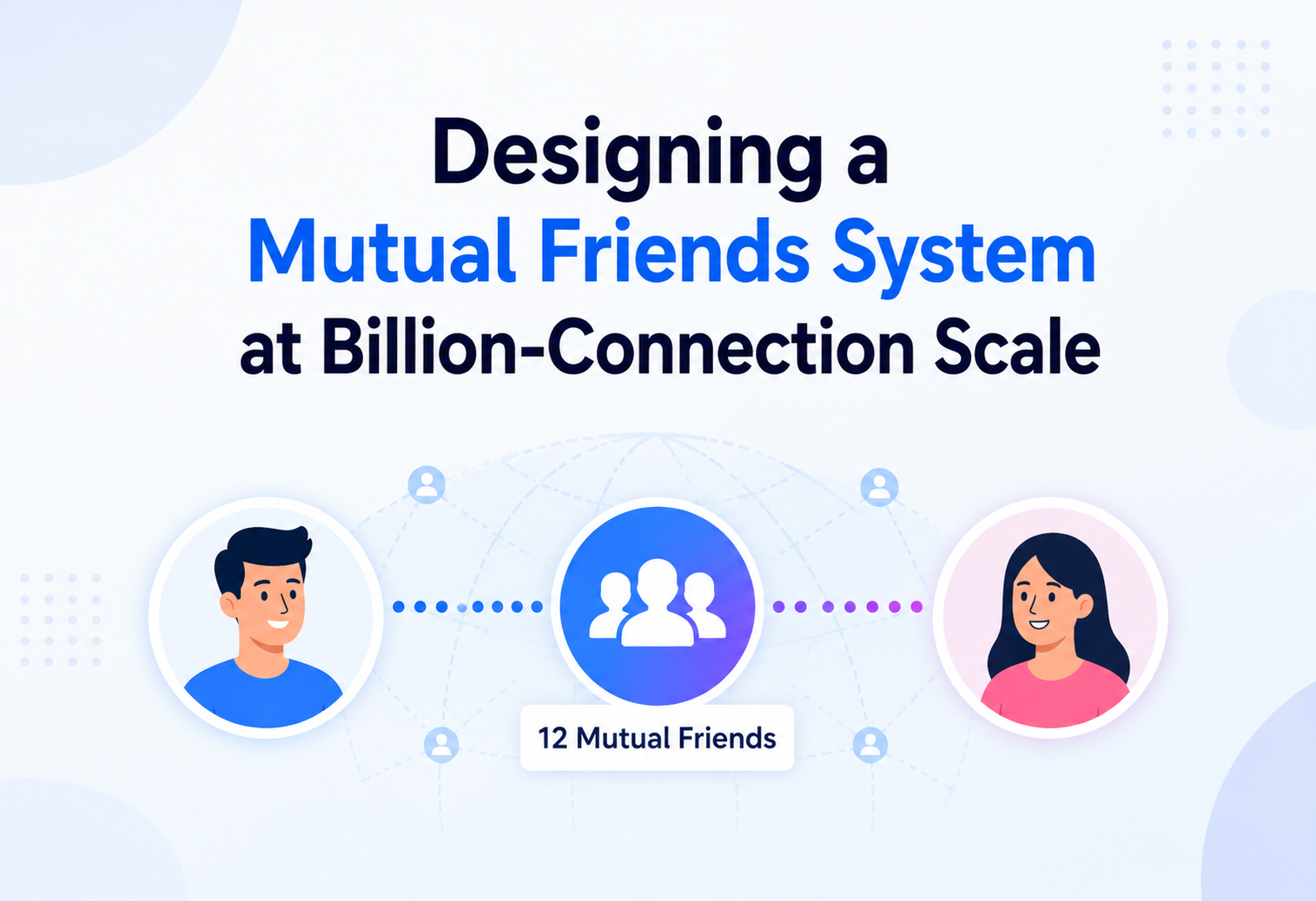
Designing a Mutual Friends System at Billion-Connection Scale
How do you tell two strangers, in under 100 milliseconds, who they both know — when the underlying graph has billions of people and hundreds of billions of edges? This is the full architecture, from adjacency lists to sharded graph stores to set-intersection algorithms that power the “People You May Know” and “X Mutual Friends” features you see on every major social network.
Introduction & History
Where the “mutual friends” idea came from, and why it quietly became one of the hardest problems in social software.
Imagine you meet someone new at a conference. Before you even exchange numbers, you both open a social app and see: “12 mutual friends.” Instantly, that stranger feels a little less like a stranger. You have a shared circle of trust. That one small feature — a number and a short list of names — is one of the most computationally expensive things a social network does at scale, even though it looks trivial on screen.
A mutual friend is simply a person who appears in the friend list (or follower/following graph) of both User A and User B. If Alice knows Bob, Carol, and Dave, and Frank knows Bob, Dave, and Eve, then Alice and Frank’s mutual friends are Bob and Dave. On paper, this is a first-year computer science exercise: intersect two sets. In production, at the scale of a network like Facebook, LinkedIn, or Instagram, it becomes a distributed-systems problem involving graph partitioning, caching, approximate algorithms, and careful engineering trade-offs.
1.1 A Short Timeline
Friendster and early Facebook. Early social networks introduced the “friend” as a bidirectional, confirmed relationship. Once two-way friendships existed, showing overlap between two people’s friend lists became a natural, almost obvious feature to build.
“People You May Know” is born. Facebook and LinkedIn independently realized that counting mutual connections was a strong signal for friend and connection recommendations. This turned a simple display feature into a core input for recommendation ranking systems, massively increasing query volume.
Graph stores emerge. As friend graphs crossed hundreds of millions of edges, relational databases buckled under adjacency-list joins. This era saw the rise of purpose-built graph and edge stores — Facebook’s TAO, LinkedIn’s early graph services, and Twitter’s FlockDB — designed specifically for fast edge lookups and set operations.
Billion-scale graphs and approximate algorithms. With billions of users and hundreds of billions of edges, exact intersection at read time became too expensive for every use case. Companies now blend exact lookups for small friend lists with probabilistic data structures (like HyperLogLog and MinHash) and precomputed, cached results for high-degree “celebrity” nodes.
Think of two people each holding a stack of business cards representing everyone they know. Finding mutual friends is like laying both stacks on a table and picking out the cards that appear in both piles. If each stack has 10 cards, a child could do this by eye in seconds. But if each stack has 5,000 cards, and you must do this instantly for millions of pairs of people simultaneously, you need a system — sorted piles, an index, or someone who has already pre-computed common cards for the busiest people ahead of time.
This tutorial walks through designing that system end to end: the data model, the storage layer, the algorithms that make intersection fast, the caching strategy that keeps popular queries cheap, and the reliability and security concerns that come with running this at the scale of a global social platform. Code examples are in Java, and every section that interviewers commonly probe is called out explicitly, since this exact problem is a favorite in system design interviews at large technology companies, both because it has a deceptively simple surface description and because a thorough answer naturally has to touch sharding, caching, algorithmic complexity, and privacy all in the same conversation.

Problem & Motivation
Why “just intersect two lists” breaks down once you’re operating at social-network scale.
At small scale, computing mutual friends is almost free. Given two friend lists of size m and n, you sort both and intersect in O(m + n) time, or use a hash set for O(m + n) average time without even sorting. A single machine can do millions of such intersections per second if the lists are small and already in memory.
The real problem is the shape of the data at scale:
Skewed Degree Distribution
Most users have a few hundred friends, but “celebrity” or highly-connected nodes (public figures, large pages, popular influencers followed by millions) can have friend/follower lists with millions of entries. A naive intersection between two such nodes is extremely expensive.
Data Doesn’t Fit on One Machine
With 3 billion users and an average of 200-plus connections each, the graph has hundreds of billions of edges. Even storing just user IDs as 8-byte integers, that’s terabytes of edge data — far beyond what a single server’s memory can hold.
Friend Lists Are Sharded Across Machines
Because the graph is partitioned (sharded) across many servers, a friend list for one user might live on Server 7, and their potential mutual friend’s list might live on Server 42. The two lists must be fetched over the network before they can be compared, adding latency.
Extremely High Query Volume
Mutual friends aren’t just shown on profile visits — they feed “People You May Know,” connection request screens, group suggestions, and messaging context. This pushes query volume into the millions per second across a large platform.
Freshness Requirements
Friendships are created and removed constantly. A stale mutual-friends count that still includes someone who unfriended both users a week ago erodes trust in the product.
Low Latency Expectations
This is usually a supporting feature on a page that must render quickly — users expect profile pages and connection lists to load in well under a second, so the mutual-friends computation gets a latency budget measured in tens of milliseconds, not seconds.
The hard part was never comparing two lists. The hard part is making sure the right two lists are ever close enough to compare in the first place. — a common framing used by graph infrastructure engineers.
“Why can’t you just run a SQL JOIN between two friend tables to get mutual friends?” A relational JOIN on a friendship table works fine for small data sets, but at billions of rows, the join has to either scan huge index ranges or perform expensive shuffles across a distributed database. It also doesn’t naturally support the access pattern of “give me this one user’s full friend list fast,” which graph stores are purpose-built for. Real systems replace the JOIN with an application-level set intersection over two pre-fetched adjacency lists, with heavy caching for repeat and high-degree queries.
2.1 Putting the Numbers in Perspective
It helps to work through the arithmetic once, because the numbers involved are easy to underestimate. Suppose a platform has 3 billion monthly active users, and each user has, on average, 300 connections. The total number of directed edges in the graph is roughly 3 billion multiplied by 300, which comes out to around 900 billion. Even representing each edge as a compact 8-byte integer, and even accounting for the fact that undirected friendships can sometimes be stored once instead of twice, the raw edge data alone runs into the terabytes. No single machine, no matter how much RAM it carries, can hold this data set in memory, which is exactly why sharding is not an optional optimization here — it is a structural requirement from day one.
Now consider query volume. If even a modest five percent of daily active users view a profile page, a friend-request screen, or a “People You May Know” module that triggers a mutual-friends computation, and each of those views triggers, say, three separate mutual-friends lookups, a platform with a billion daily active users can easily generate tens of millions of mutual-friends queries every single day, with spikes far higher during peak hours. Spread unevenly across a 24-hour period with strong regional peaks, the system regularly needs to sustain hundreds of thousands to well over a million queries per second at the busiest moments. This is the scale at which “just intersect two lists” stops being an adequate design and starts being the name of a subsystem with its own architecture, on-call rotation, and capacity planning process.
Imagine a small town library with two hundred members, where each member’s borrowing history fits on one index card. Finding out which books two members have both borrowed is trivial — you pull two cards and compare them by eye. Now imagine that same task for a national library system with three hundred million members, each with a borrowing history of hundreds of books, and millions of comparison requests arriving every second from librarians across every branch simultaneously. The task has not changed in kind, only in scale — but that change in scale is precisely what forces a complete redesign of how the data is stored, indexed, and compared.
Core Concepts
The vocabulary you need before the architecture will make sense.
3.1 The Social Graph
A social graph is a mathematical graph where each node (also called a vertex) represents a user, and each edge represents a relationship — a friendship, a follow, a connection. Facebook-style “friend” relationships are undirected (if Alice is Bob’s friend, Bob is automatically Alice’s friend). Twitter/Instagram-style “follow” relationships are directed (Alice can follow Bob without Bob following back). Mutual friends can be computed on either kind of graph, but the definition shifts slightly: for a directed graph, “mutual” might mean people that both A and B follow, or people who follow both A and B, depending on the product.
3.2 Adjacency List
The most natural way to represent “who does User X know” is an adjacency list: a mapping from each user ID to the list of user IDs they’re connected to. This is exactly the data structure needed for mutual-friend computation — you fetch User A’s adjacency list, fetch User B’s adjacency list, and intersect them.
Picture a giant phone book where, instead of phone numbers, each person’s entry lists the names of everyone they’re friends with. Alice’s entry says: “Bob, Carol, Dave.” Frank’s entry says: “Bob, Dave, Eve.” To find mutual friends of Alice and Frank, you just compare their two entries and keep the names that appear in both: Bob and Dave.
3.3 Set Intersection
Formally, if F(A) is the set of friends of user A, and F(B) is the set of friends of user B, the mutual friends of A and B are F(A) ∩ F(B), the set intersection. The count you see on screen (“14 mutual friends”) is simply |F(A) ∩ F(B)|, the size of that intersection. It is worth noting explicitly that intersection is a commutative operation — F(A) ∩ F(B) is always identical to F(B) ∩ F(A) — which is a small but useful fact, since it means the system can safely normalize the order of the two user IDs in a request before doing any work, guaranteeing that a query for “mutual friends of A and B” and a separate query for “mutual friends of B and A” always resolve to exactly the same cache entry rather than being treated, and computed, as two unrelated requests.
3.4 Graph Partitioning (Sharding)
Since the whole graph can’t live on one machine, it is split (“sharded”) across many servers. A common approach hashes the user ID to decide which shard owns that user’s adjacency list, so shard = hash(user_id) % num_shards. This means a single mutual-friends query almost always needs to talk to at least two different shards — one for each user — and sometimes more, if their friends’ data is needed too.
3.5 Fan-Out vs. Precomputation
There are two broad strategies for answering “who are A and B’s mutual friends”:
- Query-time (fan-out on read): fetch both friend lists live and intersect them when the request arrives.
- Precomputed (fan-out on write): whenever a friendship changes, update precomputed mutual-friend data for affected pairs ahead of time, so reads are just cache lookups.
Real systems use a hybrid: query-time intersection for the general case, with precomputation and heavy caching layered on top for expensive or frequently-requested pairs.
3.6 Approximate Cardinality
When you only need the count of mutual friends (not the list of names) for a very high-degree pair, computing an exact intersection can be wasteful. Probabilistic structures like HyperLogLog estimate set cardinality using a small, fixed amount of memory, trading perfect accuracy for massive space and speed savings. This matters more for aggregate analytics (“average mutual friend count across the platform”) than for a single user-facing pair, but it’s a tool worth knowing.
“What’s the difference between computing mutual friends at read time versus at write time, and when would you choose each?” Read-time (query-time) computation keeps writes cheap and data always fresh, but makes reads more expensive, especially for high-degree users. Write-time (precomputed) keeps reads cheap and fast but adds write amplification — a single new friendship can trigger updates to many cached pairs — and risks staleness if updates lag. Most production systems use read-time computation as the default, with targeted caching and precomputation only for the “hot” pairs and nodes that justify the extra write cost.
3.7 Consistent Hashing, Explained Simply
A naive way to decide which shard owns a user is shard_number = hash(user_id) % total_shards. This works, but it has a serious flaw: the moment you add or remove even a single shard, the value of total_shards changes, and almost every user’s assigned shard number changes with it. In a live system, that means almost the entire graph would need to be physically moved between machines just to add one more shard — clearly impractical at billion-user scale.
Consistent hashing solves this by arranging shard identifiers and user IDs on the same conceptual ring (a circle of hash values from 0 to some large maximum). A user is assigned to the first shard found by walking clockwise around the ring from their hashed position. When a shard is added or removed, only the small arc of the ring immediately surrounding that shard needs to be reassigned — every other user keeps their existing shard assignment. This is the same technique used inside distributed caches like Memcached clusters and inside many distributed databases, precisely because it turns an “almost everything moves” problem into a “only a small slice moves” problem.
Picture a large circular seating chart at a banquet, where each guest’s name determines a specific seat on the circle, and each table serves the guests seated in the arc nearest to it. If one table needs to be removed because it broke, only the guests who were assigned to that specific table need to be reseated at the next table along the circle — everyone else stays exactly where they are. Compare that to a seating system based on “seat number modulo number of tables,” where removing a single table would force almost every guest at the whole banquet to stand up and move.
3.8 CAP Theorem in the Context of the Friend Graph
The CAP theorem states that a distributed data store can only guarantee two of three properties at once during a network partition: Consistency (every read sees the latest write), Availability (every request gets a response, even if it might be stale), and Partition tolerance (the system keeps working despite network failures between nodes). Since network partitions are a fact of life at global scale, real systems must choose between prioritizing consistency or availability when a partition actually occurs.
For the friend graph, most production systems lean toward availability with eventual consistency for the majority of operations. If a friend request confirmation takes an extra second to propagate to every replica, that is a minor, rarely-noticed inconvenience. If a profile page fails to load because the system refused to answer during a network hiccup, that is a much more visible and damaging failure. The one place where this system leans back toward consistency, as discussed throughout this tutorial, is privacy-sensitive state such as blocking, where showing slightly-stale data can cause real harm and is treated as an exception worth extra engineering effort.

“Where does this system sit on the CAP theorem spectrum, and why?” By default, it favors availability and partition tolerance over strict consistency (an AP system), because a friend graph read that returns a few seconds of staleness is a far smaller problem than a friend graph read that fails outright. The one deliberate exception is safety-critical state like blocking, which is treated with stronger consistency guarantees and synchronous enforcement at read time, even at some cost to availability or latency, because the harm from getting that wrong is qualitatively different from ordinary staleness.
Architecture & Components
The major building blocks, and how a request flows through them.
4.1 API Gateway
The entry point for all client traffic. Handles authentication, rate limiting, request routing, and basic validation before forwarding requests to the Mutual Friends Service. It shields internal services from being directly exposed to the internet.
4.2 Mutual Friends Service
A stateless microservice responsible for orchestrating a mutual-friends request: check cache, decide if precomputed data can be used, fetch the two adjacency lists (or partial lists for very high-degree users) via the shard router, run the intersection algorithm, and return the result. Being stateless lets it scale horizontally behind a load balancer with no session stickiness required.
4.3 Graph Shard Router
A lightweight component (often a library embedded in the service, backed by a shard-mapping metadata store) that knows which physical graph store shard owns a given user’s adjacency list. It resolves user_id → shard location and fans requests out in parallel when data must be fetched from multiple shards.
4.4 Graph Store (Sharded)
The system of record for the social graph itself: who is connected to whom. Optimized for the two dominant access patterns — “give me all edges for user X” and “does an edge exist between X and Y” — rather than general-purpose relational queries.
4.5 Distributed Cache
A cache layer (typically Redis or Memcached, run as a cluster) that stores hot friend lists, precomputed mutual-friend counts for popular pairs, and serialized results for recently-requested pairs, dramatically cutting down repeated graph-store reads.
4.6 Change Data Stream
A durable, ordered event log (commonly Kafka) that publishes every friendship creation, removal, and block event. Downstream consumers — cache invalidators, the precompute service, and analytics/ML pipelines — subscribe to this stream to stay in sync without polling the graph store directly.
4.7 Precompute Service
Runs asynchronously to identify “hot” nodes (high query volume or high friend-count) and proactively computes and caches their mutual-friend relationships with frequently-paired counterparts, so the read path can skip live intersection entirely for these cases.
4.8 Profile / User Metadata Service
A separate, independently-owned service responsible for user-facing display data — names, profile photos, verification badges, and privacy settings. The Mutual Friends Service calls into it purely to enrich a resolved set of mutual-friend IDs into something presentable on screen, and never stores or duplicates that display data itself, keeping the boundary between “who is connected to whom” (the graph store’s job) and “what does this person look like to the viewer” (the profile service’s job) clean and independently scalable.
“Why is the Mutual Friends Service kept stateless, and what would go wrong if it weren’t?” Statelessness lets any instance handle any request, so the load balancer can distribute traffic evenly and instances can be added or removed without coordination or data migration. If the service held friend-list data in local memory as the source of truth, requests would need to be routed to specific instances (sticky sessions), creating hotspots for popular users, complicating deployments, and making failure recovery much harder, since a crashed instance could take unique data down with it.
Internal Working
Step by step, what actually happens when a mutual-friends request is processed.
- Request arrives at the API Gateway with two user IDs,
userAanduserB, plus the requesting user’s own ID for authorization. - Authorization check: the service confirms the requester is allowed to view this data — for example, that neither profile has restricted friend-list visibility from the requester.
- Cache lookup: the service checks the distributed cache for a key like
mutual:{min(userA,userB)}:{max(userA,userB)}(IDs are ordered so the key is consistent regardless of argument order). On a cache hit, the cached count and/or sample list is returned immediately. - Cache miss — degree check: the service asks the graph store (or a lightweight metadata cache) for the friend-count of each user. This determines the intersection strategy.
- Fetch adjacency lists: the shard router resolves the shard for each user and fetches their friend-ID lists in parallel. For most users this is a few hundred IDs; for high-degree users, this may be capped, paginated, or offloaded to a specialized path (see Section 7).
- Intersect: the smaller list is used to drive the intersection algorithm against the larger list (explained in depth in Section 7), producing the mutual set.
- Enrich: the resulting mutual friend IDs are enriched with display data (name, profile photo thumbnail) from a user-profile service or cache, since the client typically wants to render a few avatars, not just a count.
- Write-through cache: the result is stored in the cache with a short time-to-live (TTL), and/or an invalidation subscription is registered so it’s cleared when a relevant friendship changes.
- Response returned to the client: typically a count plus a small sample of mutual friend profiles, with the option to paginate the full list.
Facebook’s TAO (The Association and Objects) system models the social graph as objects and typed, bidirectional associations. A friendship is stored as a pair of associations (A→B and B→A) so that “get all friends of X” is a single, fast indexed read in either direction, without needing a join or a graph traversal at query time.
5.1 A Worked Latency Budget
It’s worth walking through a concrete latency budget for a typical request to see where the milliseconds actually go. Suppose the end-to-end target for a cache-miss request is 80 milliseconds. A realistic breakdown might allocate roughly 5 milliseconds for authorization and cache-key lookup overhead, 15 milliseconds for the parallel fetch of both users’ adjacency lists from their respective shards (dominated by network round-trip time plus shard-side lookup time, and done in parallel rather than sequentially), 10 milliseconds for the actual intersection computation itself for a typical, non-skewed pair, 20 milliseconds for enrichment calls to the profile service to fetch display names and avatar URLs for the resulting sample, and 10 milliseconds for cache write-back and response serialization, leaving roughly 20 milliseconds of headroom for the natural variance in a distributed system before the request risks breaching its target. Working through a budget like this during design, rather than only after a latency problem appears in production, helps identify which stage most needs optimization investment — in this example, the enrichment call is clearly the single largest contributor, which is exactly the kind of insight that should drive where engineering effort goes first.
This is analogous to budgeting time for a relay race before running it: a coach doesn’t just hope the team finishes in under a target time, they assign a specific target split to each leg of the race based on each runner’s known pace, so that if the team misses their overall goal, everyone already knows exactly which leg to examine first rather than guessing across the whole race.
Data Flow & Lifecycle
How a single friendship event ripples through the system, from creation to cache invalidation.
6.1 Friendship Creation
When User A accepts a friend request from User B, two things must happen atomically, or at least consistently: an edge is written to A’s adjacency list pointing to B, and an edge is written to B’s adjacency list pointing to A. This is typically done as a single write to the graph store, which internally guarantees the bidirectional write, rather than as two separate application-level writes that could partially fail.
6.2 Change Propagation
The write is published as an event onto the change-data stream: {type: "FRIEND_ADDED", userA, userB, timestamp}. Multiple consumers act on this event independently:
- Cache invalidator: proactively evicts or refreshes any cached mutual-friend entries involving A or B where the change could affect the result (commonly, entries are simply expired via TTL rather than surgically invalidated, since surgical invalidation for every affected pair is expensive at scale).
- Precompute service: if A or B is a high-degree “hot” node, schedules a background recomputation of affected precomputed pairs.
- Recommendation / ML pipeline: updates features used for “People You May Know” scoring, since a new friendship changes the mutual-friend counts that feed that model.
- Notification service: may notify users about new mutual connections, subject to their notification preferences.
6.3 Friendship Removal or Blocking
Unfriending or blocking follows the same event-driven path, but with higher urgency for cache invalidation and, in the case of blocking, an immediate visibility rule change — a blocked user must never appear in mutual-friend results shown to the blocker or vice versa, which is enforced as a hard filter at read time, not just a cache concern.
“A user blocks another user. How quickly does that need to be reflected in mutual-friends results, and how would you guarantee it?” Blocking is a privacy and safety boundary, not just a UX preference, so it should be enforced synchronously at read time regardless of cache state — the read path checks a low-latency block-list lookup (often a dedicated cache or bloom filter) before returning any result, so even a stale cache entry gets filtered. The asynchronous cache invalidation triggered by the block event is a performance optimization on top of that hard guarantee, not a substitute for it.
Algorithms & Data Structures
The actual mechanics of intersecting two friend lists efficiently — this is the heart of the system.
7.1 Choosing the Representation: Sorted Arrays vs. Hash Sets
Friend lists can be stored and fetched either as unsorted ID lists (intersect using a hash set, average O(m + n) time) or as sorted ID arrays (intersect using a two-pointer merge, O(m + n) time with excellent cache locality and no hashing overhead). Most large-scale graph stores keep adjacency lists sorted by ID, because sorted data enables far more than intersection — it also supports range queries, efficient merges, and compact delta-encoding for storage.
import java.util.*;

// Two-pointer intersection over two SORTED friend-ID arrays.
// Runs in O(m + n) time and O(1) extra space (excluding output).
public class MutualFriendsIntersector {

    public static List<Long> intersectSorted(long[] friendsA, long[] friendsB) {
        List<Long> mutual = new ArrayList<>();
        int i = 0, j = 0;

        while (i < friendsA.length && j < friendsB.length) {
            long a = friendsA[i];
            long b = friendsB[j];

            if (a == b) {
                mutual.add(a);
                i++; j++;
            } else if (a < b) {
                i++;   // advance the smaller pointer
            } else {
                j++;
            }
        }
        return mutual;
    }

    // When one list is far smaller than the other (skewed degree),
    // it's cheaper to binary-search each small-list element in the
    // large list: O(m log n) instead of O(m + n) when m << n.
    public static List<Long> intersectSkewed(long[] small, long[] large) {
        List<Long> mutual = new ArrayList<>();
        for (long id : small) {
            if (Arrays.binarySearch(large, id) >= 0) {
                mutual.add(id);
            }
        }
        return mutual;
    }

    // Adaptive dispatcher: picks the cheaper algorithm based on
    // the size ratio between the two lists.
    public static List<Long> findMutualFriends(long[] friendsA, long[] friendsB) {
        long[] small = friendsA.length <= friendsB.length ? friendsA : friendsB;
        long[] large = friendsA.length <= friendsB.length ? friendsB : friendsA;

        // Heuristic: if the large list is more than ~20x the small list,
        // binary search per element beats a linear merge.
        if (large.length > small.length * 20) {
            return intersectSkewed(small, large);
        }
        return intersectSorted(friendsA, friendsB);
    }
}
7.2 Handling Extreme Skew: The Celebrity Problem
When one side of the pair is a page or public figure followed by tens of millions of accounts, fetching and intersecting the full list on every request is wasteful and slow. Two practical mitigations:
- Roaring Bitmaps: when user IDs are dense and mapped to a compact integer space, a friend list can be represented as a bitmap where bit
iis set if useriis a friend. Intersection becomes a fast bitwise AND, and libraries like Roaring Bitmap compress these efficiently even when the data is sparse in places. - Precomputed top-K mutual pairs: for extremely high-degree nodes, the system precomputes and caches mutual-friend results for the pairs most likely to be queried (e.g., people who recently visited that profile), rather than computing on demand for arbitrary pairs.
import org.roaringbitmap.RoaringBitmap;

// Using Roaring Bitmaps for very high-degree accounts.
// Friend IDs must be mapped to a dense 32-bit integer space first.
public class BitmapIntersector {

    public static int mutualFriendCount(RoaringBitmap friendsA, RoaringBitmap friendsB) {
        // andCardinality computes |A ∩ B| without materializing
        // the full intersection set — O(number of 64-bit words), very fast.
        return RoaringBitmap.andCardinality(friendsA, friendsB);
    }

    public static RoaringBitmap mutualFriendSet(RoaringBitmap friendsA, RoaringBitmap friendsB) {
        return RoaringBitmap.and(friendsA, friendsB);
    }
}Twitter’s FlockDB, an early open-source graph store built for the follower graph, stored edges as sorted lists per user precisely so that “who does A follow” ∩ “who does B follow” style queries could use fast merge-based intersections instead of scanning a relational table.
7.3 Approximate Counting With HyperLogLog
For features that only need an approximate mutual-friend count at very large scale — such as showing “500+ mutual connections” instead of an exact number for a huge pair — a HyperLogLog sketch of each user’s friend set can estimate intersection cardinality using the inclusion-exclusion principle: |A ∩ B| ≈ |A| + |B| - |A ∪ B|, where the union is estimated by merging two HLL sketches in constant space, regardless of how large the underlying sets are.
“How would you compute mutual friends between two users where one has 50 million followers?” Avoid fetching and intersecting the full 50-million-entry list on the hot path. Options, often combined: represent very large friend/follower sets as compressed bitmaps (like Roaring Bitmaps) so intersection is a fast bitwise AND; cap the exact computation to a bounded sample or the smaller side of the pair combined with binary search into an indexed large-side structure; or fall back to an approximate cardinality estimate (HyperLogLog) when only a count, not a name list, is needed. The key insight is recognizing this as an outlier case that deserves a different code path than the median user pair.
7.4 Bloom Filters for Fast Negative Checks
A Bloom filter is a compact, probabilistic data structure that answers the question “is this element definitely not in the set, or maybe in the set?” using far less memory than storing the actual set. It can never produce a false negative, but it can occasionally produce a false positive. This asymmetry is extremely useful as a pre-filter: before doing the more expensive work of a full sorted-list intersection, the service can build (or maintain, incrementally) a Bloom filter for the larger of the two friend lists, then quickly test every element of the smaller list against it. Elements the filter confirms as “definitely not present” are discarded for free; only the small number of “maybe present” candidates need the more expensive exact check. For a small additional cost, this technique can significantly reduce wasted work when the true intersection is small relative to the size of both lists, which is the common case for two arbitrary, unrelated users.
Think of a bouncer at a club holding a rough mental picture of everyone on the guest list, without memorizing every name precisely. If someone’s name definitely doesn’t match anything in that mental picture, the bouncer can turn them away immediately with total confidence. But if a name seems plausible, the bouncer still has to check the actual printed list to be sure, because the mental picture isn’t perfectly precise. That rough mental picture, fast but occasionally uncertain, is exactly what a Bloom filter provides for data.
7.5 Complexity Comparison at a Glance
| Technique | Time Complexity | Space Overhead | Precision |
|---|---|---|---|
| Two-pointer merge (sorted lists) | O(m + n) | None beyond input | Exact |
| Binary search (skewed sizes) | O(m log n) | None beyond input | Exact |
| Roaring Bitmap AND | O(number of 64-bit words) | Compressed bitmap per user | Exact |
| Bloom filter pre-check | O(m) filter checks + exact check on candidates | ~1–2 bytes per element | Exact result, filter itself is probabilistic |
| HyperLogLog cardinality estimate | O(1) merge of fixed-size sketches | A few kilobytes per user, regardless of set size | Approximate (typically ~1–2% error) |
No single row in this table is the “correct” answer in isolation — the right choice depends on whether the caller needs an exact list or just a count, how skewed the pair’s degree is, and how tight the latency budget is for that particular request. This is exactly why the adaptive dispatcher pattern introduced earlier, choosing a strategy based on runtime characteristics of the specific request, is the practical answer used in production rather than committing to one algorithm platform-wide.
Advantages, Disadvantages & Trade-offs
Every design choice here trades something away. Naming the trade-off explicitly is what separates a good design from a lucky one.
✓ Query-Time Intersection
- Always reflects the latest friendship state — no staleness
- No write amplification; friendships are cheap to create
- Simple mental model, easy to reason about and debug
✗ Query-Time Intersection
- Read latency depends on friend-list sizes at request time
- Repeated identical queries redo the same work
- Struggles badly with high-degree “celebrity” nodes
✓ Precomputed / Cached Mutual Friends
- Reads are near-instant cache hits for hot pairs
- Predictable, low read latency at any scale
- Shields the graph store from repeated hot-key load
✗ Precomputed / Cached Mutual Friends
- Can serve stale results between updates
- Every friendship change may fan out to many cached entries
- Impossible to precompute for every possible pair — combinatorial explosion
| Approach | Read Latency | Freshness | Write Cost | Best For |
|---|---|---|---|---|
| Exact query-time intersection | Medium (10–80 ms) | Perfect | Low | Typical users, general case |
| Bitmap intersection | Low (<10 ms) | Perfect | Low-Medium | High-degree accounts |
| Cached precomputed pairs | Very low (<5 ms) | Eventually consistent | High | Hot / frequently-viewed pairs |
| Approximate (HyperLogLog) | Very low | Approximate | Low | Aggregate counts, analytics |
A well-designed system does not pick one of these; it routes each request to the cheapest approach that meets that request’s accuracy and freshness bar, escalating to more expensive strategies only when needed.
It is also worth being explicit about the trade-off between engineering complexity and marginal performance gain, since not every optimization discussed in this tutorial is worth building on day one. A team launching this feature for the first time, on a platform still measured in the low millions of users, gains very little from building a bitmap-based celebrity-account path or a full precomputation pipeline immediately — the added complexity, the additional failure modes it introduces, and the ongoing maintenance burden all outweigh a performance benefit that isn’t yet needed at that scale. The right posture is to build the simple, correct version first, instrument it thoroughly, and let real production data — actual degree distributions, actual query patterns, actual latency percentiles — decide which of these more advanced techniques earns its complexity budget, and in what order. This progressive-enhancement mindset, rather than attempting to design the fully-scaled version from the outset, is consistently how the most successful large-scale systems in this space were actually built.
Performance & Scalability
Techniques that let this system handle millions of queries per second across a billion-user graph.
| Metric | Target |
|---|---|
| Cache hit rate | ~99% |
| End-to-end latency | p99 < 100 ms |
| Core intersection cost | O(m + n) |
| Graph store shards | Thousands |
9.1 Horizontal Sharding of the Graph
Partitioning the adjacency data by hash(user_id) spreads both storage and query load evenly across many machines. Consistent hashing is preferred over plain modulo hashing so that adding or removing shards only reshuffles a small fraction of the keyspace instead of nearly all of it.
9.2 Parallel Fan-Out
When a mutual-friends request needs data from two (or more) shards, those fetches are issued in parallel, not sequentially, so total latency is close to the slower of the two calls rather than their sum.
9.3 Caching Layers
A multi-tier cache reduces load on the graph store dramatically:
- L1 — in-process cache: a small, short-TTL local cache inside each service instance for the very hottest keys, avoiding even a network hop to Redis for the busiest pairs.
- L2 — distributed cache (Redis cluster): shared across all service instances, storing recent mutual-friend results and hot friend lists.
- L3 — precomputed store: a persistent, asynchronously-refreshed store of mutual-friend data for very high-traffic pairs, effectively a materialized view.
9.4 Read Replicas
Graph store shards typically run with multiple read replicas per shard, so read-heavy mutual-friends traffic doesn’t compete with the write path (friendship creation/removal) for the same resources.
9.5 Denormalized Friend-Count Metadata
Storing each user’s friend count as a small, separately-cached field lets the service cheaply decide, before fetching any data, whether it’s dealing with a typical pair or a skewed one requiring the bitmap/approximate path.
“Your p99 latency for mutual-friends queries just spiked. Walk me through how you’d debug it.” Start by checking whether the spike correlates with cache hit rate — a drop in hit rate (e.g., after a cache node restart or a traffic pattern shift) pushes more traffic onto the graph store’s live-intersection path. Next, check for hot-key or hot-shard issues: is the spike concentrated around specific high-degree accounts or a specific shard that’s overloaded? Then check network and serialization overhead between the service and shard fetches, and confirm the adaptive algorithm dispatcher is correctly routing skewed pairs to the cheaper binary-search or bitmap path instead of a full linear merge.
9.6 Applying Little’s Law to Capacity Planning
Little’s Law states that, in a stable system, the average number of requests “in flight” (L) equals the average arrival rate of new requests (λ) multiplied by the average time each request spends in the system (W): L = λ × W. This simple relationship is extremely useful for capacity planning on the mutual-friends read path. Suppose the service must sustain an arrival rate of 500,000 requests per second, and the target average time-in-system per request (queueing plus processing) is 40 milliseconds. Little’s Law says the service must be able to hold roughly 20,000 requests in flight at once (500,000 multiplied by 0.04 seconds) without falling behind. That number directly informs how many concurrent connections, worker threads, and downstream connection-pool slots need to be provisioned — under-provisioning any of those relative to this figure causes queueing delay to balloon, which, by the same formula, further increases W and creates a feedback loop that can spiral into a full latency collapse under load.
Picture a busy coffee shop. If customers arrive at a rate of one every two seconds, and each customer takes on average one minute from ordering to walking out with their drink, Little’s Law says there will typically be about thirty customers inside the shop at any given moment. If the shop only has seating and counter space for ten people, a line will form and each customer’s total wait time will grow well beyond that one-minute average, which in turn increases how many people are inside waiting at once — the same runaway feedback loop that an under-provisioned software system experiences under load.
9.7 Connection Pooling
Every call from the Mutual Friends Service to a graph store shard, a cache node, or the profile-enrichment service happens over a network connection. Establishing a brand-new TCP connection (and, for encrypted traffic, completing a TLS handshake) for every single request adds latency that is entirely wasted overhead, often larger than the actual useful work being done. Connection pooling solves this by keeping a warm set of already-established connections to each downstream dependency, reused across many requests, with the pool sized according to the concurrency levels derived from Little’s Law above. Pools are typically configured with a minimum size to keep some connections always warm, a maximum size to avoid overwhelming a downstream shard, and health checks that evict and replace connections that go stale or start erroring.
public class GraphShardClientConfig {
    private static final int MIN_POOL_SIZE = 50;
    private static final int MAX_POOL_SIZE = 500;
    private static final int CONNECT_TIMEOUT_MS = 50;
    private static final int REQUEST_TIMEOUT_MS = 30;

    // Pool sizing here is derived from expected concurrency via Little's Law,
    // not chosen arbitrarily — undersizing causes queueing, oversizing wastes
    // memory and file descriptors on both client and shard.
    public ConnectionPool buildPool(String shardHost) {
        return ConnectionPool.builder()
            .host(shardHost)
            .minConnections(MIN_POOL_SIZE)
            .maxConnections(MAX_POOL_SIZE)
            .connectTimeoutMs(CONNECT_TIMEOUT_MS)
            .requestTimeoutMs(REQUEST_TIMEOUT_MS)
            .build();
    }
}High Availability & Reliability
Mutual friends is a supporting feature, but it appears on high-traffic pages — it must degrade gracefully, never take the whole page down.
10.1 Replication
Every graph store shard is replicated across multiple nodes, typically across availability zones, so the loss of a single machine or even an entire zone doesn’t make that shard’s data unavailable.
10.2 Graceful Degradation
If the graph store or a specific shard is slow or unavailable, the Mutual Friends Service should return a best-effort, possibly stale, cached result rather than an error, or omit the mutual-friends count entirely on the page rather than failing the whole profile load. A missing “12 mutual friends” line is a minor cosmetic issue; a failed profile page is not.
10.3 Timeouts and Circuit Breakers
Calls to graph store shards are bounded by aggressive timeouts (tens of milliseconds), and a circuit breaker trips if a shard is consistently failing, routing traffic to cached/fallback data instead of repeatedly hammering an unhealthy shard.
public class MutualFriendsService {

    public MutualFriendsResult getMutualFriends(long userA, long userB) {
        try {
            MutualFriendsResult cached = cache.get(cacheKey(userA, userB));
            if (cached != null) return cached;

            return circuitBreaker.executeWithFallback(
                () -> computeLive(userA, userB),
                throwable -> staleFallback(userA, userB)  // last-known-good cache entry
            );
        } catch (Exception e) {
            // Never fail the whole page render for this feature.
            return MutualFriendsResult.empty();
        }
    }
}
10.4 Disaster Recovery
The graph store maintains regular snapshots plus a replayable write-ahead log (or relies on the durable change-data stream) so that in a catastrophic event, a region can be rebuilt from backups and replayed events rather than being permanently lost. Multi-region replication further protects against a full regional outage, at the cost of eventual consistency across regions for the most recent writes.
Treating the mutual-friends path as critical-path infrastructure and letting its failures cascade into full page failures. This feature should always be an optional, best-effort enhancement to a page, wrapped in its own failure boundary.
10.5 Quorum-Based Replication
Rather than requiring every replica of a graph store shard to acknowledge a write before it’s considered successful (which would make the system only as available as its least reliable replica), most designs use a quorum approach: a write is acknowledged once a majority of replicas confirm it, and a read can similarly be satisfied by a majority. This means the system tolerates the failure of a minority of replicas without any interruption to reads or writes, while still providing strong-enough consistency guarantees for the friend graph’s needs. The exact quorum sizes (commonly expressed as N replicas, W required for a write, R required for a read) are tuned based on how strongly the system wants to favor read latency, write latency, or consistency for a given class of data — privacy-sensitive edges like blocks may use stricter quorum settings than ordinary friendships.
10.6 Chaos Testing
Because this system must survive shard failures, network partitions, and cache outages gracefully, those failure modes are deliberately and regularly exercised in a controlled way rather than only being discovered during a real incident. Chaos testing practices — killing random shard replicas, injecting artificial latency into cache calls, or simulating a full cache cluster outage during a staging load test — validate that circuit breakers trip correctly, fallbacks return sensible defaults, and the rest of the page continues to render even when this particular subsystem is fully degraded. Teams that skip this step often find that their theoretically-graceful degradation logic has a bug that only surfaces the first time it’s actually needed, which is the worst possible time to discover it.
“How would you test that your graceful degradation logic actually works, before it’s needed in a real incident?” Through deliberate chaos engineering in a staging or canary environment: kill shard replicas, inject latency and errors into cache and graph-store calls, and confirm the service still returns a valid, if degraded, response within its latency budget and never propagates an exception up to the page render. This is paired with automated regression tests around the circuit breaker’s trip and reset thresholds, and periodic game-day exercises where the on-call team practices responding to a simulated shard outage, so both the code and the humans operating it are validated before a real failure occurs.
Security
Mutual friends data touches privacy directly — it reveals relationships between people who never asked to be compared.
11.1 Authorization and Visibility Rules
Every request must respect each user’s friend-list visibility setting. If User A has set their friend list to “Only Me,” their entries should never surface in someone else’s mutual-friends computation, even indirectly, regardless of who’s asking.
11.2 Blocking Is Absolute
As covered in Section 6, if either user has blocked the other, or if a mutual-friend candidate has blocked one of the two users being compared, that candidate must be excluded from the result — enforced synchronously, not just eventually through cache expiry.
11.3 Rate Limiting and Scraping Prevention
Mutual-friends endpoints are a favorite target for scrapers building shadow social graphs (for spam, ad targeting, or deanonymization). Per-user and per-IP rate limiting, anomaly detection on query patterns (e.g., one account querying mutual friends against thousands of distinct target users in a short window), and CAPTCHAs or step-up authentication for suspicious patterns all help mitigate this.
11.4 Data Minimization
APIs should return only what the UI needs — a count and a small sample — rather than the full mutual-friend list by default, reducing the value of any single scraped response and limiting blast radius if an endpoint is abused.
11.5 Encryption and Access Control
Graph store data is encrypted at rest and in transit (TLS between all internal services). Access to raw graph store APIs is restricted to authenticated internal services via mutual TLS or short-lived service tokens — no client ever talks to the graph store directly.
“How would you prevent someone from scraping mutual-friends data to build a shadow map of the entire social graph?” Layer defenses rather than relying on one control: strict per-account and per-IP rate limits on the endpoint, behavioral anomaly detection that flags accounts querying an unusually large number of distinct target pairs, requiring the requester to actually have some relationship to at least one of the two users being queried where the product allows it, returning bounded/sampled data instead of full lists by default, and step-up challenges (CAPTCHA, temporary throttling, or account review) when anomalous patterns are detected.
11.6 Insider Threat and Least-Privilege Access
Not every security threat comes from outside the company. Because the graph store holds highly sensitive relationship data for billions of people, access to it internally is governed by the principle of least privilege: engineers and internal tools are granted only the specific, narrow access they need for their actual job function, not broad standing access to raw graph data. Production access to query arbitrary users’ friend lists directly, bypassing the service layer’s authorization checks, is typically restricted to a very small number of highly-audited break-glass tools, each access to which is logged, time-limited, and requires a documented justification and, often, a second approver. Every such access is recorded in an immutable audit log that security teams review, both proactively and in response to any reported incident, so that misuse — whether accidental or malicious — can be detected and investigated after the fact even if it wasn’t blocked in the moment.
11.7 Encryption Key Management
Data encrypted at rest is only as secure as the management of the keys used to encrypt it. Production systems typically use a dedicated key management service (KMS) that generates, rotates, and controls access to encryption keys separately from the data they protect, so that a compromise of the storage layer alone does not automatically expose readable data. Keys are rotated on a regular schedule, and old data can be re-encrypted under new keys during that rotation, limiting how much historical data any single compromised key could expose. This separation of concerns — data storage in one system, key custody in another, with tightly controlled and audited communication between them — is a standard defense-in-depth practice across nearly all systems handling sensitive personal data, and the social graph is no exception.
Assuming that encryption at rest alone is sufficient protection. Encryption at rest defends against a narrow threat — someone gaining access to raw disks or backups — but does nothing against a compromised, over-privileged service account, an unaudited internal tool, or a misconfigured access policy that lets legitimate credentials read far more than they should. Defense in depth, combining encryption, strict access control, auditing, and rate limiting, is what actually protects this data.
Monitoring, Logging & Metrics
You cannot operate a system at this scale by intuition — you need continuous, structured visibility into its behavior.
12.1 Key Metrics to Track
Latency Percentiles
p50, p95, p99, and p999 latency for the mutual-friends endpoint, broken down by cache-hit vs. cache-miss path.
Cache Hit Rate
Per cache tier (L1/L2/L3), since a drop here directly predicts a load increase on the graph store.
Shard Load Balance
Requests and latency per graph store shard, to catch hot shards caused by skewed data or a “viral” account.
Error and Timeout Rate
Split by failure type (timeout, circuit breaker open, shard unavailable) to speed up root-cause analysis.
Intersection Algorithm Path
Ratio of requests served by the linear-merge path vs. the binary-search/skewed path vs. the bitmap path, confirming the adaptive dispatcher is behaving as expected.
Staleness / Lag
Time between a friendship-change event and its reflection in cache invalidation, to catch a lagging or backed-up change stream.
12.2 Logging
Structured logs (JSON) for every request include a trace ID, the two user IDs (hashed or tokenized for privacy in long-term storage), which cache tier served the result (if any), latency breakdown per stage, and any fallback path taken. Distributed tracing (e.g., via OpenTelemetry) ties together the gateway, service, cache, and shard calls for a single request into one trace for debugging.
12.3 Alerting
Alerts are set on symptom-level signals users actually feel — elevated p99 latency, elevated error rate, dropping cache hit rate — rather than only on low-level causes, so on-call engineers are paged for things that matter and can use dashboards to drill into cause once paged.
Large-scale graph systems commonly run dedicated dashboards showing a live heat map of shard load, so an operator can visually spot a single overloaded shard (often caused by a viral post or account) before it triggers cascading timeouts elsewhere in the system.
12.4 Service Level Objectives and Error Budgets
Rather than chasing perfection, mature teams define an explicit Service Level Objective (SLO) for this feature — for example, “99.9% of mutual-friends requests complete successfully within 150 milliseconds, measured over a rolling 30-day window.” This target is deliberately looser than 100%, because it acknowledges that some small level of failure is both inevitable at this scale and acceptable given the feature’s non-critical nature. The gap between the SLO and perfect reliability is the error budget — a quantified, spendable allowance for things going wrong. When the error budget is healthy, the team has room to take calculated risks: ship a riskier optimization, run a more aggressive chaos test, or roll out a new caching strategy faster. When the error budget is nearly exhausted, the team shifts focus toward stability work and slows down the pace of risky changes until reliability recovers. This turns an abstract goal like “be reliable” into a concrete, trackable number that directly informs day-to-day engineering priorities.
12.5 Dashboards Built for Different Audiences
A single monitoring dashboard rarely serves everyone well. An on-call engineer responding to a page needs a small number of high-signal panels — current error rate, current p99 latency, recent deploys — that let them assess “is this bad, and did we just cause it” within seconds. A capacity planner needs longer-range trend views — request volume growth over months, shard storage growth, cache hit-rate trends — to forecast when more shards or cache nodes will be needed. Product and analytics stakeholders often want a different view entirely, focused on how mutual-friends data feeds into recommendation quality rather than raw system health. Building distinct, purpose-built dashboards for each of these audiences, rather than one dashboard trying to serve all three, meaningfully speeds up both incident response and planning work.
“How would you define a good SLO for this feature, and why does it matter?” A good SLO is specific, measurable, and tied to what users actually experience — for instance, a latency and success-rate target measured from the client’s perspective over a meaningful rolling window, not an internal implementation metric like “cache hit rate,” which is a means to an end rather than the end itself. It matters because it turns reliability into a concrete, trackable budget rather than an open-ended, unachievable goal of zero failures, which in turn gives the team a principled, data-driven way to decide when to prioritize new features versus stability work.
Deployment & Cloud
How this system is packaged, rolled out, and run in production cloud environments.
13.1 Containerized, Stateless Services
The Mutual Friends Service and shard router are packaged as containers and run on an orchestrator (Kubernetes is typical), which handles horizontal auto-scaling based on CPU, request rate, or custom latency-based metrics, and automatically replaces unhealthy instances.

13.2 Multi-Region Deployment
The service layer is deployed in multiple regions close to major user populations, reducing round-trip latency. The graph store itself is partitioned with region-aware placement where possible, keeping a user’s data close to where they’re most often accessed from, while maintaining cross-region replicas for durability and failover.
13.3 Progressive Rollouts
Changes to the intersection algorithm, cache TTLs, or shard routing logic are rolled out using canary deployments — a small percentage of traffic first — with automated rollback if latency or error-rate metrics regress, since a subtle bug in the hot intersection path can affect an enormous fraction of platform traffic almost immediately.
13.4 Infrastructure as Code
Shard topology, cache cluster configuration, and scaling policies are defined declaratively (e.g., Terraform) and version-controlled, so infrastructure changes are reviewed, auditable, and reproducible across environments.
13.5 Cost Optimization
At this scale, infrastructure cost is a first-class design constraint, not an afterthought. A few practical levers matter more than any single clever algorithm. First, cache hit rate has an almost direct, linear relationship with graph-store cost: every percentage point of cache hit rate improvement removes a proportional slice of expensive backend reads, which is why caching investment tends to have the best cost-to-benefit ratio of anything in this system. Second, right-sizing compute — using auto-scaling policies tuned to real traffic patterns rather than permanently provisioning for peak load — avoids paying for idle capacity during the long stretches of a day that aren’t at peak. Third, storage tiering matters for the graph store itself: very cold, rarely-accessed edges (for example, connections belonging to long-inactive accounts) can be moved to cheaper, slower storage tiers, while hot data for active users stays on fast, more expensive storage. Finally, choosing compact binary serialization formats (rather than verbose text-based formats like JSON) for internal service-to-service traffic reduces both network bandwidth costs and CPU time spent on serialization, which matters enormously when multiplied across millions of requests per second.
It is common for large-scale platforms to report that caching investments — improving hit rate on hot read paths like this one — deliver some of the single highest returns on engineering investment anywhere in the infrastructure stack, precisely because the cost of a cache hit is often several orders of magnitude lower than the cost of the equivalent live computation against a sharded backend store.
Databases, Caching & Load Balancing
Choosing the right storage engines and traffic-distribution strategy for graph-shaped data.
14.1 Why Not a Plain Relational Database?
A relational database can model friendships as rows in a table with two foreign keys. This works at modest scale, but “get all friends of X” becomes an index range scan that competes with all other write and read traffic on shared tables, and cross-shard joins for mutual-friend computation are notoriously expensive to plan and execute well in most RDBMS engines at this scale.
14.2 Purpose-Built Graph / Edge Stores
Systems like Facebook’s TAO or a custom key-value store optimized for edge lists store data with the access pattern baked in: a primary key of (user_id, edge_type) maps directly to a sorted list of connected IDs, so “get friends of X” is a single, fast point lookup rather than a scan or join.
| Storage Option | Strength | Weakness |
|---|---|---|
| Relational DB (sharded) | Strong consistency, familiar tooling | Expensive joins, harder to scale writes |
| Wide-column store (e.g., Cassandra-style) | Great for sorted adjacency lists, linear scale-out | Eventual consistency by default, needs careful key design |
| Purpose-built graph/edge cache (TAO-style) | Optimized exactly for this access pattern, very fast reads | More custom infrastructure to build and operate |
| Native graph database | Rich traversal queries (friends-of-friends, paths) | Can be harder to shard linearly at extreme scale |
14.3 Caching Strategy
As covered in Section 9, a multi-tier cache (in-process → distributed → precomputed store) is essential. Cache keys are normalized (smaller user ID first) so mutual(A,B) and mutual(B,A) hit the same entry. TTLs are tuned per tier — shorter for L1, longer for L2 — with event-driven invalidation layered on top for correctness-sensitive cases like blocking.
14.4 Load Balancing
At the edge, a global load balancer or GeoDNS routes clients to their nearest region. Within a region, an application-layer load balancer distributes traffic across stateless service instances using a low-latency algorithm (such as least-outstanding-requests) rather than simple round robin, which handles uneven per-request cost (a celebrity-pair query vs. a typical one) far better.
“Would you use a relational database, a NoSQL store, or a dedicated graph database for the friend graph, and why?” At billion-user scale, a purpose-built edge/adjacency store (conceptually similar to a wide-column store or a system like TAO) usually wins, because the dominant access pattern — fetch all edges of one node, fast — doesn’t need general-purpose relational query flexibility or full graph-traversal power. A native graph database shines for deep, complex traversal queries (friends-of-friends-of-friends, shortest paths), but those aren’t the core mutual-friends use case, and native graph databases have historically been harder to horizontally scale to hundreds of billions of edges than simpler key-value-shaped stores.
14.5 Replication Factor and Durability Trade-offs
Every shard of the graph store is stored with a replication factor — typically three copies in production social-graph systems — spread across different physical racks or availability zones. A replication factor of three tolerates the simultaneous loss of any single copy (due to hardware failure, a bad deployment, or a zone outage) while still keeping the shard fully readable and writable from the surviving two copies. Going higher, to a replication factor of five, buys additional durability and read capacity at the cost of more storage and more write coordination overhead, since a write must propagate to more replicas before being considered durable. Most teams find three to be the practical sweet spot for this workload: enough redundancy to survive realistic failure scenarios, without the operational and storage cost of over-replicating data that changes relatively infrequently per user.
14.6 Rebalancing Shards as the Graph Grows
Even with consistent hashing minimizing the disruption, shard rebalancing is still an operation that must be handled carefully. When a new shard is added to absorb growing data volume, the system gradually migrates the affected slice of user data to the new shard in the background, typically using a dual-write or shadow-read strategy during the transition: writes go to both the old and new location temporarily, and reads are gradually shifted over once the new shard’s data is confirmed complete and consistent, before the old copy is finally decommissioned. This kind of live migration, performed on a data store serving live production traffic, is one of the more delicate operational tasks in running this system, and is usually automated and throttled so it never competes meaningfully with live query traffic for the same resources.
Large-scale distributed data stores commonly perform these migrations at a deliberately throttled pace — moving only a small percentage of total capacity per hour — specifically so that background rebalancing traffic never competes with, or degrades, live user-facing query latency, even though this means a full rebalance across a very large cluster can take days to complete.
APIs & Microservices
How this capability is exposed to clients and consumed by other internal services.
15.1 Public-Facing API
// Request
GET /v1/users/{userId}/mutual-friends?withUser={otherUserId}&limit=6

// Response 200 OK
{
  "count": 14,
  "sample": [
    { "userId": "9f2a...", "displayName": "Bob Chen",  "avatarUrl": "..." },
    { "userId": "3b7d...", "displayName": "Dave Kumar", "avatarUrl": "..." }
  ],
  "hasMore": true,
  "nextCursor": "eyJvZmZzZXQiOjZ9"
}
The API returns an exact or approximate count plus a small paginated sample rather than the full list by default, both for performance and for the data-minimization reasons discussed in Section 11.
15.2 Internal Service-to-Service API
Internally, a gRPC interface is typically preferred over REST/JSON between the Mutual Friends Service and the graph store, for lower serialization overhead and strongly-typed contracts on the hot path.
service GraphService {
  rpc GetFriendIds(FriendListRequest) returns (FriendListResponse);
  rpc GetFriendCount(FriendCountRequest) returns (FriendCountResponse);
}

message FriendListRequest {
  int64 user_id = 1;
  int32 max_results = 2;
  string page_cursor = 3;
}

message FriendListResponse {
  repeated int64 friend_ids = 1;
  string next_cursor = 2;
  bool has_more = 3;
}
15.3 Microservice Boundaries
The Mutual Friends Service is intentionally kept separate from the core Graph/Friendship Service that owns writes, so read-heavy mutual-friends traffic can be scaled, cached, and evolved independently without risking the correctness-critical write path for friendships themselves. It’s also separate from the Profile Service (which owns names, photos) — the mutual-friends response is enriched by calling that service, rather than duplicating profile data into the graph store.
Letting the Mutual Friends Service write directly to the graph store, or letting the core Friendship Service also own intersection logic. Mixing read-optimized and write-optimized concerns in one service makes both harder to scale and reason about independently.
15.4 API Versioning and Backward Compatibility
As the mutual-friends API evolves — adding new fields, changing the shape of the sample payload, or introducing new query parameters — it must not break existing client applications that may take weeks or months to update, particularly mobile apps that update on their own release cadence rather than the backend’s. The API is versioned explicitly in its path (as seen in the example above, /v1/...), and new, non-breaking fields can be added to existing response payloads freely, since well-behaved clients ignore fields they don’t recognize. Any genuinely breaking change — removing a field, changing a field’s meaning, or changing an existing status code’s behavior — requires a new version path, with the old version kept alive and fully functional until client adoption of the new version reaches a level where deprecation of the old one is safe. This discipline is what allows the backend team to keep improving the system continuously without being blocked on, or accidentally breaking, every client that consumes this API.
15.5 Idempotency for Internal Write Paths
While the mutual-friends read path has no writes of its own, the underlying friendship creation and removal events it depends on must be idempotent, since the change-data stream and its consumers operate under an at-least-once delivery guarantee rather than an exactly-once one — a network retry or consumer restart can cause the same event to be delivered and processed more than once. Each friendship-change event carries a unique identifier, and every consumer (the cache invalidator, the precompute service, the recommendation pipeline) tracks which event identifiers it has already processed, so that reprocessing the same event a second time is a safe no-op rather than a source of duplicated side effects, such as double-decrementing a precomputed mutual-friend count.
“The change-data stream occasionally delivers the same friendship-added event twice. How does the system stay correct?” By designing every consumer of that stream to be idempotent with respect to the event’s unique identifier — tracking processed event IDs and skipping duplicates — rather than assuming the stream provides exactly-once delivery, which most durable, high-throughput streaming systems intentionally do not guarantee because doing so would come at a steep cost to throughput and availability. This is a standard, well-understood trade-off in distributed systems: it is far cheaper and more robust to make consumers idempotent than to try to make the delivery mechanism perfectly exactly-once.
Design Patterns & Anti-Patterns
Recurring solutions worth reusing, and recurring mistakes worth avoiding.
16.1 Patterns to Apply
Cache-Aside
The service checks cache first and only computes on a miss, then writes the result back — simple, robust, and the default pattern for this system’s read path.
CQRS (Command Query Responsibility Segregation)
Friendship writes go through the core Graph/Friendship Service; mutual-friends reads go through a separate, independently-scaled service — separating the two responsibility paths entirely.
Event-Driven Invalidation
Cache and precomputed data are kept fresh via the change-data stream rather than by polling, decoupling producers and consumers of friendship-change events.
Adaptive Algorithm Selection
The intersection strategy (merge, binary search, bitmap) is chosen dynamically based on input size, rather than hardcoding one approach for all pairs.
Circuit Breaker
Protects the graph store from cascading overload when a shard is degraded, and protects the calling service from piling up slow requests.
Bulkhead Isolation
The mutual-friends read path is resource-isolated (separate thread pools/connection pools) from other features so a spike in this feature’s load can’t starve unrelated functionality, and vice versa.
16.2 Anti-Patterns to Avoid
Synchronous Full-Graph Joins
Running a live join across the entire friendship table for every request doesn’t scale past a small user base and blocks on lock contention under write load.
Unbounded Precomputation
Trying to precompute mutual friends for every possible pair of users is combinatorially impossible — with 3 billion users, the number of pairs vastly exceeds any feasible storage budget. Precompute selectively.
Cache Stampede
When a popular cache entry expires, many concurrent requests can simultaneously miss and hammer the graph store at once. Mitigate with request coalescing or jittered TTLs.
Ignoring Skew
Treating every pair of users identically, using the same intersection algorithm regardless of degree, guarantees poor tail latency once a request touches a high-degree account.
“What is a cache stampede, and how does it apply here?” A cache stampede happens when a popular cache entry expires and a burst of concurrent requests for that same key all miss the cache at once, each independently falling through to recompute the expensive result and hammering the backing store simultaneously. For a viral profile pair (e.g., two people who just went viral together), this can spike graph-store load sharply. Mitigations include request coalescing (only one in-flight computation per key, with other requests waiting on that result), staggered/jittered TTLs so entries don’t all expire at once, and proactively refreshing hot keys slightly before they expire.
16.3 Observer Pattern for the Change Stream
The relationship between the graph store and its downstream consumers — the cache invalidator, the precompute service, the recommendation pipeline, and the notification service — follows the classic Observer pattern, generalized to a distributed setting via the change-data stream. The graph store, as the subject, does not need to know anything about who is listening or what they do with each friendship-change event; it simply publishes the event once. Each interested consumer subscribes independently and reacts in whatever way suits its own purpose, at its own pace. This decoupling is what allows new consumers to be added later — for example, a future analytics pipeline studying friendship-formation patterns — without requiring any change at all to the graph store’s write path, since the publisher and its subscribers are never directly coupled to one another.
16.4 Request Coalescing in Practice
Request coalescing, mentioned above as a stampede mitigation, deserves a closer look because it is one of the more commonly misunderstood patterns in this space. The idea is straightforward: when the service detects that a computation for a given cache key is already in flight (triggered by an earlier, concurrent request for the same pair), any additional requests for that same key are not allowed to independently trigger their own redundant computation. Instead, they attach themselves to the already-running computation and simply wait for its result once it completes, and all of them receive the same answer. This is typically implemented with an in-memory map of “in-flight futures” keyed by cache key, guarded by appropriate concurrency controls, and cleaned up once the underlying computation resolves. The benefit compounds with popularity: for an extremely hot pair experiencing thousands of simultaneous requests during a stampede window, only one of those requests actually does the expensive work, while the other thousands wait a few milliseconds for that single result rather than each independently repeating the same costly computation against the backing graph store.
This same coalescing pattern is used broadly across high-traffic systems well beyond social graphs — for example, in content delivery networks handling a sudden burst of requests for the same newly-published, not-yet-cached asset, where only the first request actually fetches from the origin server and every other concurrent request for that same asset simply waits for and reuses that one fetch’s result.
Best Practices & Common Mistakes
Lessons that separate a system that survives launch day from one that survives five years of growth.
17.1 Best Practices
- Design for the tail, not the average. Median friend-list sizes are small; the system’s cost and complexity are driven almost entirely by the small fraction of high-degree accounts.
- Keep the read path independently scalable from the write path. Separate services, separate resource pools, separate failure domains.
- Make every failure mode degrade gracefully. A missing mutual-friends count should never break a page.
- Normalize cache keys (ordered user IDs) so equivalent queries always hit the same cache entry.
- Instrument the algorithm dispatcher so you can see, in production, which intersection strategy is actually being used and how often.
- Treat blocking and privacy settings as hard, synchronous constraints, never something that can lag behind via eventual consistency.
- Load test with realistic, skewed degree distributions, not uniformly-sized synthetic friend lists, since uniform test data hides the exact problems that show up in production.
17.2 Common Mistakes
- Assuming friend lists are small. Designs that only work for a few hundred friends fall over the first time they meet a public figure’s account.
- Over-precomputing. Trying to cache every possible pair leads to unsustainable storage growth and write amplification.
- Under-caching. Recomputing identical, frequently-repeated queries from scratch wastes enormous graph-store capacity.
- Coupling reads and writes in one service, making it impossible to scale or deploy them independently.
- Forgetting pagination on the mutual-friends list, forcing large payloads for high-count pairs.
- Skipping privacy enforcement on cached data, serving a stale result that includes a user who has since blocked or restricted visibility.
Optimizing purely for average-case latency in benchmarks that don’t reflect the real, highly-skewed degree distribution of a production social graph — this is one of the most common gaps between a system design that looks good on paper and one that survives contact with real traffic.
17.3 A Pragmatic Rollout Checklist
Teams that have shipped systems like this successfully tend to follow a similar sequence rather than attempting a single, all-at-once launch. Start with a correct, simple, single-shard-friendly implementation validated against real production-shaped test data, including a realistic long-tail of high-degree accounts, not just uniformly-sized synthetic friend lists. Add caching early, since it is both the highest-leverage optimization and the one most likely to reveal key-normalization and invalidation bugs while the system is still small enough to debug easily. Introduce sharding and the adaptive algorithm dispatcher once real traffic and real degree-distribution data are available to validate the skew thresholds against, rather than guessing those thresholds up front. Layer in graceful degradation, circuit breakers, and chaos testing before, not after, the feature reaches significant traffic, since retrofitting resilience into a system already under load is far riskier than building it in from the start. Finally, instrument thoroughly and define SLOs before declaring the system “done,” since a feature without clear reliability targets tends to accumulate invisible technical debt that only surfaces during an incident.
“If you had to launch a first version of this system quickly, what would you deliberately leave out, and what would you never skip?” Safe to defer initially: bitmap-based intersection for extreme celebrity accounts, cross-region multi-master replication, and elaborate precomputation for hot pairs — these are scaling refinements that can be added once real traffic data shows exactly where they’re needed. Never safe to skip, even in a first version: correct enforcement of blocking and privacy visibility rules, basic rate limiting to prevent scraping, and a graceful fallback path so a backend hiccup never fails the whole page. Those are the elements where getting it wrong causes real user harm or reputational damage, not just a performance regression that can be fixed later.
Real-World / Industry Examples
How this problem has actually been solved by companies operating at this scale.
Facebook / Meta — TAO
TAO models the social graph as objects and bidirectional associations with a geographically-distributed caching layer in front of a sharded MySQL storage layer. Friend edges are stored so that fetching all edges of a node is a single fast operation, making mutual-friend intersection straightforward once both lists are fetched. TAO’s read-heavy caching design directly informed how many later graph systems approached this problem.
LinkedIn — Mutual Connections at Professional Scale
LinkedIn’s connection graph feeds mutual-connection counts into both profile pages and connection-request flows, where mutual connections are a strong trust signal in a professional context. LinkedIn has published on its use of specialized graph-serving infrastructure and heavy caching to keep this feature fast across a large, highly-connected professional network.
Twitter — FlockDB
FlockDB, open-sourced by Twitter, was a distributed graph database purpose-built for storing large adjacency lists (followers, following) with fast set operations like intersection and union, explicitly designed for exactly this kind of query pattern rather than general graph traversal.
Instagram — “Following” Overlap
Instagram surfaces overlap in who two accounts follow as a discovery and trust signal, built on similar principles: a sharded follow-graph store, aggressive caching, and special handling for very high-follower accounts.
Across all of these systems, the same underlying shape recurs: a purpose-built, sharded edge store optimized for “fetch all edges of one node” as the primary access pattern, a caching layer absorbing the vast majority of read traffic, and special-cased handling for the small number of extremely high-degree nodes that would otherwise dominate system cost.
18.1 What These Systems Have in Common — and Where They Differ
Looking across these examples, three shared design decisions stand out as close to universal at this scale. First, none of them rely on a general-purpose relational database as the primary store for the friend or follower graph itself once the platform passes a modest size — the access pattern mismatch between “give me all edges of one node, fast” and what relational engines are optimized for becomes too costly to ignore. Second, every one of them treats caching not as an optional performance tweak but as a core architectural layer that the rest of the system is designed around, since the economics of serving hundreds of millions of daily active users make a high cache hit rate the difference between a sustainable infrastructure bill and an unsustainable one. Third, every one of them has, at some point in its evolution, needed to build special-cased handling for extremely high-degree accounts, because a generic design that treats every node identically inevitably breaks down at the long tail.
Where they differ is largely in how directed the underlying relationship is, and what that implies for the definition of “mutual.” Facebook and LinkedIn’s core relationships are bidirectional and symmetric by construction — a confirmed friend or connection is mutual by definition on both sides the moment it’s created — which simplifies some aspects of the data model. Twitter and Instagram’s follow relationships are asymmetric, meaning the system must be explicit about which of several possible definitions of “mutual” a given product surface is using, and must fetch the correct one of the following-list or follower-list for each user depending on that definition. This distinction, more than any difference in raw engineering sophistication, is often the biggest source of subtlety when adapting a design like this from one type of platform to another.
Frequently Asked Questions
Related but not identical. Mutual friends compares two specific, already-known users. “Friends of friends” (used for “People You May Know”) is a broader traversal: for a single user, find all second-degree connections and rank them, often using mutual-friend count between the target user and each candidate as one input signal among many. In practice, the mutual-friends intersection logic described throughout this tutorial is frequently reused as a building block inside that larger recommendation pipeline, computed for many candidate pairs at once as part of a batch scoring job rather than as a single real-time user-facing request, which is a good example of how the same core algorithm can serve two quite different products with two very different latency and consistency requirements.
The number of user pairs grows quadratically with user count. For 3 billion users, the number of possible pairs is astronomically larger than any feasible storage system, and only a tiny fraction of pairs are ever actually queried. Precomputing everything wastes essentially all of the effort; computing on demand with caching for the pairs that are actually requested is far more efficient.
The core intersection algorithm is identical, but “mutual” needs a precise definition: it could mean accounts both A and B follow, accounts that follow both A and B, or some combination. Each definition pulls from a different adjacency list (following-list vs. follower-list), so the system needs to fetch the correct list for the specific product definition being used.
If the sharding scheme happens to co-locate both users’ adjacency lists on the same shard, the fetch can be done as a single local call instead of two parallel remote calls, saving a network round trip. Some systems intentionally try to co-locate frequently-interacting users on the same shard for exactly this reason, though this must be balanced against overall load distribution.
This generalizes to intersecting more than two sets: fetch all N friend lists and intersect them pairwise, ideally starting with the smallest lists first to shrink the working set as early as possible. For large groups this gets expensive quickly, so real products typically cap the group size or only compute this on demand for small groups (e.g., a group chat’s “friends you all know”).
Yes. Relationship data is personal data under regulations like GDPR. Users generally have rights to control visibility of their friend list, and the system must honor deletion/right-to-be-forgotten requests by removing a user’s edges from the graph store and purging any cached or precomputed data derived from them, not just their primary profile record.
Test the pure algorithm functions in isolation with a range of inputs: empty lists, one empty list, fully identical lists, fully disjoint lists, and lists of wildly different sizes to exercise the skew-detection threshold. Separately, test the dispatcher’s routing decision by asserting which underlying algorithm is invoked for a given pair of input sizes, using mocks or spies rather than re-verifying correctness of each algorithm again at that layer. Property-based testing — generating many random pairs of sorted arrays and asserting the result always matches a trusted, simple reference implementation — is particularly effective at catching edge cases a hand-written test suite might miss.
This is a product and privacy decision as much as a technical one. Many platforms restrict relationship data, including mutual-friend counts, to authenticated users, since showing it to anonymous visitors both weakens the ability to enforce per-viewer visibility rules and increases the risk of large-scale scraping by automated, unauthenticated clients. Where it is shown to logged-out visitors, it typically comes with much stricter rate limiting and a smaller default result set.
Returning the first few IDs found during intersection, in raw storage order, tends to produce an arbitrary and unhelpful sample. Production systems typically rank the intersected set by a relevance signal — such as how recently the viewer interacted with each mutual friend, how close in the graph they are, or a general engagement or closeness score already computed for other product features — and return the top-ranked few. This turns a mechanically-correct feature into one that actually feels useful, since a mutual friend the viewer talks to daily is a far more meaningful thing to surface than one they haven’t interacted with in years.
Summary & Key Takeaways
The Core Ideas to Carry Forward
- Mutual friends is fundamentally a set intersection problem, but scale transforms it into a distributed-systems and algorithms problem simultaneously.
- The social graph must be sharded, with a purpose-built edge store optimized for “fetch all edges of one node” as the dominant access pattern.
- Skewed degree distribution — a small number of extremely high-degree accounts — drives most of the system’s real-world complexity and cost.
- An adaptive intersection strategy (sorted merge, binary search for skewed pairs, bitmap AND for extreme cases) keeps both typical and outlier queries fast.
- A multi-tier cache, invalidated by an event-driven change stream, absorbs the overwhelming majority of read traffic and protects the graph store.
- Privacy and blocking rules are hard constraints enforced synchronously at read time — never something allowed to lag behind through eventual consistency.
- The feature must be built to degrade gracefully: it is a supporting element on high-traffic pages and should never be allowed to fail the whole page.
- Real systems (Facebook’s TAO, Twitter’s FlockDB, LinkedIn’s graph infrastructure) converge on the same shape: sharded edge storage, heavy caching, and special-cased handling for high-degree nodes.
Ultimately, the mutual friends feature is a useful case study precisely because it looks deceptively simple on the surface while touching nearly every major theme in distributed systems design: partitioning data too large for one machine, choosing between consistency and availability under realistic failure conditions, picking the right algorithm for a skewed real-world input distribution, caching aggressively without sacrificing correctness on privacy-sensitive edges, and building operational practices — monitoring, SLOs, chaos testing — that keep the whole thing healthy long after the initial launch. Anyone who can design this system well, end to end, has effectively demonstrated fluency in the core skills that large-scale backend engineering actually demands day to day, which is exactly why it remains such a durable and popular question in system design interviews.
“Just intersect two lists” is a first-year computer science exercise. What makes this system a favorite interview question is that every layer above the intersection — where the lists live, how they get to the same machine in time, how the result gets cached, how blocks and privacy are enforced, and how the whole thing keeps working when one shard misbehaves — is where the actual engineering happens. The intersection is easy. Everything around it is the system.