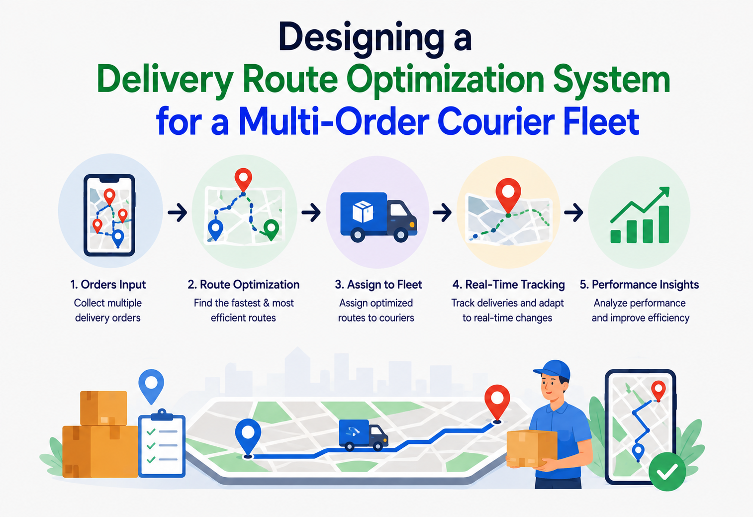
Designing a Delivery Route Optimization System for a Multi-Order Courier Fleet
How platforms with hundreds of couriers — each juggling several simultaneous orders — decide who picks up what, in what order, and along which route, balancing delivery speed, fairness, and fleet-wide efficiency at scale. A full architectural walkthrough from continuous order ingestion and geospatial pre-filtering, through fast heuristic matching, per-courier route sequencing, anytime local-search improvement, real-time re-optimization, graceful degradation, and observability.
Introduction & History
Every food-delivery, parcel-courier, or last-mile logistics platform eventually runs into the same deceptively hard question: given hundreds of couriers already on the road right now, each one already carrying one or more orders, and a continuous stream of new orders arriving every few seconds, who should pick up and deliver what, and in what sequence, so that every order arrives as fast as possible without wearing the fleet — or the business’s margins — down?
This is not a new problem invented by app-based delivery companies. It is a modern, real-time instance of one of the oldest and most studied problems in operations research: the Vehicle Routing Problem (VRP), itself a generalization of the even older Traveling Salesman Problem (TSP), first rigorously studied in the 1950s and 60s by researchers at RAND Corporation and elsewhere working on military and industrial logistics.
The TSP asks: given a set of locations, what is the shortest possible route that visits each one exactly once and returns to the start? It is famously NP-hard — the time required to find the guaranteed-optimal answer grows explosively with the number of locations, making exact solutions computationally infeasible beyond a fairly small number of stops. The VRP extends this to multiple vehicles, each with capacity constraints, time windows, and starting or ending depots, and remains just as computationally hard (arguably harder), since the problem now includes deciding which stops go to which vehicle in addition to the ordering within each vehicle’s route.
Think of the shift manager at a large pizza chain with fifty branches across a city, watching a wall of live orders scroll in every minute. For every new order she has to answer, in seconds: which branch bakes it, which of the delivery riders on that branch takes it, and if that rider is already carrying two other orders, in what order do they visit the three houses? Multiply that decision by hundreds of couriers, thousands of restaurants, and millions of orders a day, and you have the problem this guide is about — the same “who serves this, in what order, and along which route” question, only continuously, in real time, at fleet scale.
1.1 A short history: from overnight batch runs to sub-second decisions
For decades, VRP solving was primarily a batch, offline planning exercise. Logistics companies like UPS and FedEx would compute delivery routes for their trucks the night before, or the morning of a shift, using powerful but slow optimization solvers, because the inputs (which packages, which addresses) were largely known in advance and vehicles ran fixed routes for the whole day.
The rise of on-demand, app-based courier platforms in the 2010s (Uber Eats, DoorDash, Instacart, Grubhub, and similar international platforms) fundamentally changed the shape of the problem. Orders now arrive continuously and unpredictably throughout the day, couriers are already mid-route when new orders appear, and the acceptable time to compute a “good enough” answer shrank from overnight batch runs to a small number of seconds — because a customer waiting for food doesn’t care that the underlying optimization problem is NP-hard. They just want an accurate, fast delivery estimate and a courier who shows up promptly.
This shift — from offline, batch VRP solving to online, continuous, real-time re-optimization under hard latency constraints — is the central engineering challenge this tutorial focuses on. It is not “how do we solve the TSP or VRP” in the abstract mathematical sense (a well-studied field with decades of algorithmic research), but “how do we build a production system that continuously, approximately, and fast enough re-solves a live, ever-changing version of this problem for hundreds of couriers simultaneously.”

It combines a genuinely hard, well-known algorithmic problem (VRP/TSP, both NP-hard) with real-time systems constraints, geospatial data structures, and a rich set of competing business objectives (speed vs. fairness vs. cost vs. courier earnings) — giving a candidate room to demonstrate both algorithmic literacy and pragmatic systems judgment about when to approximate rather than solve exactly.
1.2 Setting expectations up front: nobody “solves” VRP in production
It is worth setting expectations clearly up front: no production system in this space “solves” the Vehicle Routing Problem in the rigorous, provably-optimal sense that an operations-research textbook means by that phrase. Every real platform discussed in this tutorial makes a deliberate, well-understood trade-off — accepting a fast, good-enough approximate answer over a slow, exact one — because in this domain, a courier who receives their next instruction in half a second with a route that is 8% longer than theoretically optimal is a vastly better outcome than a courier waiting twenty seconds for a provably perfect answer.
Internalizing this trade-off early is arguably the single most important framing decision for approaching this entire problem space, both in a real engineering context and in a system design interview discussion. If you take nothing else from this section, take this: the goal is not the optimal answer — the goal is the best answer we can produce inside the time we have.
1.3 Who this guide is for
This guide is written for engineers, students, and interview candidates who already understand basic web application concepts (clients, servers, databases, message queues) but want a thorough, from-first-principles walkthrough of how a real, production-grade real-time route optimization system is designed and reasoned about. Every technical term used is introduced with a plain-English definition, a real-life analogy, and a concrete example, so no prior background in operations research or logistics is assumed. By the end, you should be able to not only describe the architecture from memory, but explain the specific failure mode each component exists to prevent — which is exactly what a strong system design interview answer requires.
Architecture & Components
The system needs to do five things, continuously and in parallel. (1) Ingest new orders and up-to-the-second courier location/status updates. (2) Decide, for each new or re-evaluated order, which courier should serve it and where in that courier’s current multi-stop route it should be inserted. (3) Compute an efficient sequence of pickups and drop-offs for each courier carrying multiple simultaneous orders. (4) Continuously re-optimize as real-world conditions change (traffic, cancellations, new orders, a courier going offline). (5) Turn the resulting plan into clear, turn-by-turn guidance for each courier’s app.
flowchart TB
    ORDERS["Incoming Orders Stream"] --> INGEST["Order Ingestion Service"]
    LOC["Courier Location and Status Updates"] --> TRACK["Courier State Tracker"]
    INGEST --> MATCH["Matching and Assignment Engine"]
    TRACK --> MATCH
    MATCH --> ROUTE["Route Sequencing Engine
per-courier stop ordering"]
    ROUTE --> ETA["ETA Prediction Service"]
    ROUTE --> DISPATCH["Dispatch Service"]
    DISPATCH --> COURIERAPP["Courier Mobile App"]
    ETA --> CUSTAPP["Customer App
live tracking"]
    MATCH --> GEOIDX["Geospatial Index
courier and order locations"]
    ROUTE --> MAPSVC["Map and Routing Service
road network, travel times"]
    TRACK --> REOPT["Continuous Re-optimization Trigger"]
    REOPT --> MATCH
    MATCH --> STORE[("Assignment and Route State Store")]
    DISPATCH --> METRICS["Fleet Metrics and Monitoring"]
2.1 Core Components
| Component | Responsibility |
|---|---|
| Order Ingestion Service | Accepts new orders as they are placed, normalising pickup location (restaurant/warehouse), drop-off location, time constraints (ready time, promised delivery window), and any special handling requirements before pushing them into the matching pipeline. |
| Courier State Tracker | Maintains real-time knowledge of every courier’s current location, current in-progress route and carried orders, remaining capacity, and availability status, fed by frequent location pings from the courier app. |
| Geospatial Index | An indexed spatial data structure (commonly a geohash grid, quadtree, or R-tree) enabling fast “which couriers are near this order” and “which orders are near this courier” queries. Essential, since naive distance computation against every courier for every order does not scale. |
| Matching & Assignment Engine | Decides which courier should be assigned a given new order (or re-evaluates existing assignments), balancing proximity, current load, and route efficiency against fairness and delivery-time promises. |
| Route Sequencing Engine | Given a courier’s current set of assigned orders (potentially several, picked up from different locations and destined for different drop-offs), computes an efficient sequence of stops — this is the per-courier “mini-VRP” that determines the actual order in which pickups and drop-offs happen. |
| Map / Routing Service | Provides real road-network travel time and distance estimates between any two points, typically backed by a licensed or self-hosted routing engine using live traffic data — the ground truth the optimization algorithms reason about rather than straight-line distance. |
| ETA Prediction Service | Combines route sequencing output with historical and real-time data (traffic, restaurant prep time patterns, courier-specific speed tendencies) to produce accurate delivery time estimates shown to customers. |
| Continuous Re-optimization Trigger | Periodically or event-drivenly re-evaluates active assignments and routes as conditions change — new orders appear, couriers deviate from plan, or an order is cancelled — deciding whether the current plan is still good enough or needs adjustment. |
| Dispatch Service | Translates the current optimized plan into concrete instructions pushed to each courier’s app: next pickup, next drop-off, turn-by-turn navigation handoff. |
2.2 How the components fit together as a card grid
Order & Location Streams
Two continuous feeds — new orders and courier location pings — drive everything downstream. Both are high-throughput, event-driven, and must never block the matching path.
Matching + Sequencing
Matching answers “which courier?” and sequencing answers “in what order does that courier visit their stops?” — two related but distinct sub-problems, deliberately separated.
Geospatial Index + Map Service
Fast proximity queries prune the candidate set; the routing engine gives real, traffic-aware travel times so the algorithm reasons about the road network, not straight lines.
Dispatch + ETA
The plan becomes real once dispatched to the courier’s app; the ETA service turns the same plan into a live tracking experience for the waiting customer.
- “Why do you need a separate geospatial index instead of just querying courier locations from a regular database?” — a regular relational or document database has no efficient way to answer “which of these hundreds of couriers are within 2 km of this point” without scanning many rows and computing distance for each; a geospatial index (geohash / quadtree / R-tree) supports this as a fast, indexed range query, which matters enormously once matching must run repeatedly, in real time, at fleet scale.
- “Why separate the Matching Engine from the Route Sequencing Engine instead of one combined component?” — matching (which courier gets which order) and sequencing (in what order does that courier visit their stops) are related but distinct sub-problems with different scopes and update frequencies. Separating them lets each be optimized, scaled, and re-triggered independently — for example, a minor traffic change might only require re-sequencing a courier’s existing stops without re-running the more expensive fleet-wide matching decision.
Internal Working
This is where the interesting engineering lives. Below we walk through why the problem is genuinely NP-hard, why production systems accept “good enough” over “optimal,” and how the actual matching and sequencing pipeline handles a new order arriving at, say, 12:47:03 on a Friday lunch rush.
3.1 Why this is genuinely NP-hard, and what that means in practice
The core reason this problem is hard is combinatorial explosion. For a single courier carrying just 4 orders (4 pickups and 4 drop-offs, with the constraint that each pickup must precede its corresponding drop-off), there are already thousands of valid orderings to choose from. For a whole fleet of hundreds of couriers being matched against a continuous stream of orders, the number of possible assignment-and-sequencing combinations is astronomically larger than anything an exact algorithm could enumerate and evaluate within a real-time latency budget.
This is precisely why production systems do not attempt to find the mathematically optimal solution — they use fast, well-understood heuristic and metaheuristic algorithms that find a very good (not provably optimal) solution within a strict time budget. This is a completely standard and expected trade-off in this problem domain, not a shortcut or compromise unique to any one company’s implementation.
3.2 Constructive heuristics: building an initial plan fast
The first step is usually a fast, greedy construction algorithm that produces a reasonable starting solution in milliseconds:
- Nearest neighbor / greedy insertion: for a new order, evaluate candidate couriers (typically pre-filtered by the geospatial index to a nearby subset, not the entire fleet) and insert the new pickup/drop-off pair into whichever courier’s existing route sequence produces the smallest increase in total route cost (time or distance), subject to feasibility constraints (capacity, time windows).
- Savings algorithm (Clarke-Wright, adapted): a classic VRP construction heuristic that starts from individual point-to-point routes and iteratively merges routes together where doing so produces the largest “savings” in total travel distance, adapted in modern systems to account for capacity and time-window constraints.
These constructive heuristics are deliberately simple and fast — their job is to get to a workable, decent plan almost instantly, not to be the final answer.
3.3 Improvement heuristics: polishing the plan
Once an initial feasible plan exists, local-search improvement techniques refine it further within the remaining time budget:
- 2-opt / Or-opt moves: classic TSP-improvement techniques that consider swapping the order of two stops, or relocating a small segment of stops to a different position in the route, keeping the swap only if it reduces total route cost — cheap to evaluate and effective at removing obviously inefficient “crossing paths” in a route.
- Simulated annealing / tabu search / large neighborhood search: more sophisticated metaheuristics that allow temporarily accepting a worse solution to escape local optima, within a bounded computation budget. These are commonly used for the more complex multi-courier, multi-constraint re-optimization passes rather than the fastest real-time single-order insertion path.
The practical engineering discipline here is anytime algorithms: the optimization process is designed so that it always has a valid, usable answer available, and simply keeps improving that answer for as long as it is given time to run. If the system needs an answer in 200 ms because a courier’s app is waiting for the next instruction, it takes whatever the algorithm has produced so far; if there is a slightly larger time budget available (for example, a less time-sensitive batch re-optimization pass), the same algorithm keeps refining and produces a better answer.
“The goal is not the optimal answer — it is the best answer we can produce inside the time we have. Anytime algorithms make that trade explicit and controllable.”
3.4 Constraints the algorithm must respect
| Constraint | Why it matters |
|---|---|
| Precedence (pickup before drop-off) | An order’s drop-off stop can never be sequenced before its own pickup stop — a hard constraint every candidate route must satisfy. |
| Capacity | A courier (especially on a bike or scooter with a limited-size delivery bag) can only carry a bounded number of simultaneous orders or bounded total volume/weight. |
| Time windows | Food orders often have a narrow acceptable delivery window driven by food-quality concerns (hot food should not sit for 40 minutes); package deliveries may have customer-requested or SLA-driven windows. |
| Pickup readiness time | An order cannot actually be picked up until the restaurant or warehouse has finished preparing it — arriving too early just means the courier waits, which is itself a cost the sequencing algorithm should account for. |
| Courier-specific constraints | Vehicle type (bike vs. car vs. scooter affects speed and route options, e.g. bikes can use paths cars cannot), working-hours limits, and any courier-stated preferences the platform chooses to honor. |
3.5 Batching: deciding which orders to combine
A related but distinct decision from route sequencing is order batching: given a courier already en route with capacity to spare, should a new nearby order be added to their current run, or should it wait for a courier who can serve it alone, faster? Batching improves fleet-wide efficiency (fewer total courier-miles per order, lower cost per delivery) but can slightly slow down the individual orders being batched together, since a courier now has to make multiple stops instead of going directly to one destination. This is one of the sharpest trade-offs in the whole system, and is discussed in more depth in the trade-offs chapter.
flowchart LR
    NEWORDER["New Order Arrives"] --> FILTER["Geospatial Filter
nearby eligible couriers"]
    FILTER --> CANDIDATES["Candidate Couriers
small subset of fleet"]
    CANDIDATES --> EVAL["Evaluate insertion cost
per candidate route"]
    EVAL --> FEASIBLE{"Feasible given
capacity and time windows?"}
    FEASIBLE -->|No| EVAL
    FEASIBLE -->|Yes| BEST["Select lowest
marginal-cost insertion"]
    BEST --> ASSIGN["Assign order and update
courier route sequence"]
    ASSIGN --> IMPROVE["Local-search improvement
2-opt / Or-opt pass"]
    IMPROVE --> FINAL["Updated route pushed
to courier"]
- “Would you try to find the mathematically optimal route for each courier?” — no. Given the NP-hard nature of the problem and the real-time latency budget, production systems use fast constructive heuristics plus bounded local-search improvement (anytime algorithms), deliberately trading provable optimality for a good-enough answer within a strict time budget. A candidate who insists on exact optimization here is missing a core, well-established trade-off in this problem space.
- “How would you decide whether to batch a new order onto an already-busy courier’s route versus assigning a dedicated courier?” — compare the marginal insertion cost (added time and distance, and impact on existing orders’ promised delivery times) against the fleet-wide efficiency gain and the availability of a faster dedicated alternative. This is fundamentally a policy decision with tunable weights, not a fixed rule, and should be explicitly named as a business trade-off.
3.6 Objective function: what “best” actually means
A crucial and often underappreciated design decision is that “optimal” is not a single, self-evident target — it is a weighted combination of multiple, sometimes competing objectives that the business must explicitly define and tune. A typical objective function combines terms such as:
- Total courier travel time or distance across the fleet (efficiency).
- Individual order lateness relative to promised delivery time (customer experience).
- Courier idle time or utilization balance (fairness and earnings).
- The cost of any pickup wait time where a courier arrives before an order is ready (wasted courier time).
These terms are combined into a single scalar cost that the heuristic algorithms are actually trying to minimize, with relative weights that reflect real business priorities — for example, weighting on-time delivery heavily during a promotional period focused on customer trust, or weighting courier idle-time fairness more heavily in a market where courier retention is a pressing concern. Because these weights are ultimately business and product decisions rather than purely technical ones, a well-designed system exposes them as tunable configuration rather than hardcoding a single fixed objective function, allowing the platform to adapt its optimization priorities by market, time of day, or business initiative without requiring an algorithm rewrite.
3.7 Look-ahead and anticipatory matching
The simplest version of matching is purely reactive: an order arrives, and the system immediately decides which courier serves it based on current state. More sophisticated systems incorporate a degree of anticipatory reasoning — for example, deliberately holding a courier momentarily idle near a location with historically high order density (a popular restaurant cluster right before a predictable lunch rush) rather than immediately dispatching them on a marginal, less efficient order, because doing so improves expected fleet-wide efficiency over the next several minutes even though it looks locally suboptimal in the instant.
This kind of anticipatory positioning draws on ideas from reinforcement learning and predictive demand modeling, and represents a meaningfully more advanced (and more operationally risky, since it depends on demand forecasts being reasonably accurate) layer on top of the reactive matching and sequencing techniques that form the foundation of most production systems. It is worth naming as a natural “what would you do next” extension in a deeper interview discussion, while being clear that reactive, real-time matching is the necessary foundation any such anticipatory layer builds on top of, not a replacement for it.
Data Flow & Lifecycle
Let’s walk through the full lifecycle of one order, from the moment a customer taps “place order” to the moment the courier taps “delivered.” This is where the abstract components in Chapter 2 start behaving as a coordinated pipeline.
4.1 New order arrival
- An order is placed and enters the Order Ingestion Service with its pickup location, drop-off location, and any timing constraints.
- The Geospatial Index is queried to identify a small candidate set of nearby, available (or soon-to-be-available) couriers, rather than considering the entire fleet — this pruning step is essential for keeping the subsequent evaluation fast.
- For each candidate courier, the Matching Engine evaluates the marginal cost of inserting this new order’s pickup/drop-off pair into that courier’s current route at every feasible position, using the Route Sequencing Engine’s insertion-cost evaluation logic.
- The courier (and insertion position) with the lowest marginal cost, subject to all hard constraints being satisfied, is selected, and the assignment is recorded.
4.2 Continuous re-optimization
- As couriers move, new orders arrive, and conditions change (traffic, cancellations), the Continuous Re-optimization Trigger periodically (or on significant events) re-evaluates whether the current fleet-wide plan is still good, or whether a better arrangement now exists — for example, swapping which of two nearby couriers serves which of two nearby pending orders, if their relative positions have shifted enough to make the swap beneficial.
- Re-optimization is deliberately scoped and bounded — it does not re-solve the entire fleet’s assignments from scratch on every trigger, but rather considers a local neighborhood of potentially-improvable assignments (e.g., orders and couriers within a certain geographic and temporal proximity of each other), keeping the computation tractable at fleet scale.
4.3 Route execution and dispatch
- The Dispatch Service continuously pushes the courier’s next instruction (go to this pickup, or this drop-off) to their app, updating as the underlying route sequence changes due to re-optimization.
- As the courier completes each stop (confirmed via the app, often combined with GPS geofencing to detect arrival), the Courier State Tracker updates their current position in the route, freeing capacity and potentially triggering a fresh round of matching or re-optimization for their now-partially-emptied route.
4.4 Handling disruptions
- If an order is cancelled mid-route, it is removed from the courier’s sequence and the remaining stops are re-sequenced if beneficial.
- If a courier goes offline unexpectedly (app crash, connectivity loss, or explicit sign-off) while still carrying active orders, those orders must be quickly reassigned to another nearby courier — a scenario requiring careful handling since the original courier may have already physically picked up the items, which the reassignment logic and the customer-facing communication must account for.
sequenceDiagram
    participant Order as New Order
    participant Geo as Geospatial Index
    participant Match as Matching Engine
    participant Route as Route Sequencing Engine
    participant Courier as Courier App
    participant Track as Courier State Tracker

    Order->>Geo: Query nearby couriers
    Geo-->>Match: Candidate courier list
    Match->>Route: Evaluate insertion cost per candidate
    Route-->>Match: Best insertion and cost
    Match->>Match: Select lowest marginal-cost courier
    Match->>Track: Update assigned courier route state
    Match->>Courier: Push updated route and next stop
    Courier->>Track: Confirm stop completion (geofence + tap)
    Track->>Match: Trigger re-optimization check (capacity freed)
- “A courier goes offline mid-delivery with two active orders still in their bag. What happens?” — the system detects the disconnect (missed heartbeat or location pings beyond a threshold), flags those orders as needing reassignment, and — since the physical items are already with the original courier — this typically requires operational fallback (contacting the courier directly, or in the worst case, cancelling and refunding or re-ordering) rather than a purely algorithmic reassignment. This is an important real-world edge case to name rather than assume away.
Advantages, Disadvantages & Trade-offs
Every meaningful design choice in this system is a trade-off — not a mistake, and not a solved problem, but a permanent tension the platform tunes explicitly. The table below names the five sharpest ones.
| Aspect | Advantage | Disadvantage / Trade-off |
|---|---|---|
| Order batching (multiple orders per courier) | Reduces total courier-miles and cost per delivery, improving fleet-wide efficiency and courier earnings per hour. | Individual orders within a batch may take slightly longer than if served by a dedicated courier, directly trading fleet efficiency against individual delivery speed. |
| Heuristic / approximate optimization | Meets strict real-time latency requirements at fleet scale, where exact optimization is computationally infeasible. | Produces “good enough,” not provably optimal, routes — some inefficiency relative to a theoretical best-case solution is an accepted, permanent cost of operating in real time. |
| Frequent re-optimization | Adapts quickly to changing conditions (traffic, cancellations, new nearby orders), keeping the plan close to locally optimal as the world changes. | Frequent route changes can be disorienting or frustrating for couriers if not carefully bounded (a courier being redirected repeatedly mid-route erodes trust in the system), and adds computational load. |
| Geospatial pre-filtering before matching | Makes matching computationally tractable by avoiding evaluation of clearly irrelevant, far-away couriers. | An overly aggressive filter radius can exclude a courier who would actually have been the best match (e.g., one who is slightly farther away but moving in a very favorable direction), requiring careful tuning. |
| Fairness-aware assignment | Distributing orders more evenly across the fleet improves courier satisfaction and retention. | Pure fairness optimization can conflict with pure efficiency optimization (the “best” courier for an order, purely by proximity or route-cost, is not always the one who has been idle longest), requiring an explicit, tunable balance between the two objectives. |
None of these trade-offs resolves cleanly in favor of one side. The right balance for any given platform depends on its specific market dynamics, competitive pressures, and stage of growth, and mature systems typically expose these balances as configurable, monitored policy levers rather than baking a single fixed answer into the algorithm itself.
Treat every one of these trade-offs as a dial the business owns, not a decision the algorithm silently makes. The engineering job is to expose the dial cleanly and monitor what happens as it moves; the business job is to decide where to point it this month.
Performance & Scalability
Everything in this chapter follows from one number: the latency budget. Once you know how many milliseconds you have to answer “who takes this order,” every other choice — geospatial pre-filtering, zone partitioning, travel-time caching — becomes obvious.
6.1 The latency budget
Matching a new order to a courier typically needs to complete within a few hundred milliseconds to a couple of seconds — fast enough that the customer sees a near-instant order confirmation and estimated delivery time. This tight budget is what fundamentally shapes the algorithmic choices described in Chapter 3: there simply is not time for exhaustive search, which is why geospatial pre-filtering (reducing the candidate set from hundreds of couriers to a handful of realistic nearby options) is not just a performance optimization but a structural necessity for making the subsequent optimization computation tractable within budget.
6.2 Scaling matching across a large fleet and service area
At city or regional scale, the matching problem is naturally decomposable geographically — a courier in one part of a city is essentially never a realistic candidate for an order in a distant part of the same city, so the system can partition its active state (couriers, pending orders) into geographic cells or zones (commonly using a geohash-based grid) and run matching computation independently, in parallel, per zone, with only modest coordination needed at zone boundaries (an order or courier near a boundary may need to consider candidates from an adjacent zone as well).
This geographic partitioning is the primary lever for horizontal scalability, letting the system add compute capacity per zone as order density grows in that zone, rather than needing every matching decision to reason about the entire fleet at once.
6.3 Balancing re-optimization frequency against compute cost
Re-optimizing continuously and exhaustively for every fleet member on every location update would be prohibitively expensive at scale. Production systems instead use triggered, scoped re-optimization — re-evaluating only when a meaningful event occurs (new order, cancellation, significant courier deviation from plan) and only within a bounded local neighborhood of potentially-affected couriers and orders, rather than a global recomputation. This keeps the average computational cost proportional to the rate of meaningful real-world change, not to the total fleet size squared, which would be the cost of naively re-evaluating all possible reassignments across the whole fleet on every update.
6.4 Precomputing and caching travel times
Repeatedly calling a full routing engine for live, turn-by-turn travel time between every candidate courier-order pair on every matching decision is expensive. Systems commonly maintain a cache of recent travel-time estimates between frequently-relevant location pairs (e.g., a popular restaurant to nearby delivery zones), refreshed periodically or upon significant traffic pattern shifts, and fall back to a live routing engine call only when a fresh, uncached estimate is genuinely needed — trading a small amount of estimate staleness for a large reduction in the load placed on the routing engine, which is itself often a rate-limited or cost-metered external or internal dependency.
flowchart TB
    CITY["City Service Area"] --> Z1["Zone A
geohash cell cluster"]
    CITY --> Z2["Zone B"]
    CITY --> Z3["Zone C"]
    Z1 --> M1["Matching compute
Zone A couriers and orders"]
    Z2 --> M2["Matching compute
Zone B couriers and orders"]
    Z3 --> M3["Matching compute
Zone C couriers and orders"]
    M1 -.->|Boundary overlap check| M2
    M2 -.->|Boundary overlap check| M3
- “How would you scale matching computation as the fleet grows into the thousands across many cities?” — geographic partitioning (zones or geohash cells) so matching computation is independently parallelizable and scoped, since couriers and orders in distant zones are never realistic candidates for each other. This turns an otherwise fleet-size-dependent computation into one that scales with per-zone order density instead.
- “What would you do if the routing engine dependency became a bottleneck under load?” — caching frequently-needed travel-time estimates, falling back to straight-line-distance-based heuristics with a correction factor for cases where a fresh, precise estimate is not strictly necessary (e.g., initial coarse candidate filtering before the final precise evaluation), and applying request coalescing and rate limiting to protect the routing engine from redundant concurrent calls for near-identical route queries.
6.5 Illustrative capacity numbers
These numbers are illustrative rather than prescriptive, since actual figures depend heavily on city density, order volume patterns, and the specific vehicle mix (bikes, scooters, cars) in a given market — but working through a concrete estimate like this in an interview setting demonstrates the ability to reason quantitatively about scale rather than treating “hundreds of couriers” as an unquantified abstraction.
High Availability & Reliability
The cost of failure here is felt by real people in real time — a courier standing confused at the wrong location, or a customer’s order silently stuck unassigned. That framing shapes every reliability decision below.
- Graceful degradation of optimization quality: if the Matching or Route Sequencing Engine is under unusually heavy load or a dependency (like the routing engine) is degraded, the system should fall back to faster, simpler heuristics (e.g., pure nearest-neighbor assignment without local-search improvement) rather than failing to assign orders at all — a slightly less efficient route is far preferable to no route.
- Redundant, regionally-distributed matching compute: since matching is naturally partitioned by geographic zone, the failure of compute serving one zone should not affect other zones, and each zone’s matching workload should be able to fail over to healthy compute capacity within acceptable latency.
- Stale-location tolerance: courier location updates can occasionally be delayed or missed (poor connectivity); the system should tolerate brief staleness gracefully (continuing to use the last-known position with appropriate uncertainty) rather than treating a courier as unavailable the moment a single location ping is late.
- Idempotent dispatch instructions: if a dispatch message to a courier’s app is retried due to a transient network issue, it must not cause duplicate or conflicting instructions to appear — dispatch messages should be versioned/sequenced so a courier’s app can safely ignore an out-of-date or duplicate instruction.
These reliability practices matter more here than in many other systems precisely because the cost of failure is felt by real people in real time — a courier standing confused at the wrong location, or a customer’s order silently stuck unassigned, are tangible, immediate failures rather than abstract system metrics. This is a useful framing for why this domain tends to invest heavily in graceful degradation relative to systems where a temporary degraded state is less consequential.
Designing the matching and routing pipeline so that any dependency failure (a routing engine timeout, a geospatial index hiccup) results in an order simply not being assigned is a serious reliability gap in a system where “no assignment” directly means a customer’s order sits unfulfilled. Every stage of the pipeline needs an explicit, tested fallback path — even a suboptimal one — because a degraded assignment is almost always better than none.
- “What happens to order assignment if your primary routing or matching compute for a zone goes down entirely?” — failover to redundant compute capacity for that zone (since zones are independently scaled and can be run with standby capacity), combined with a fallback to simpler, faster heuristics if even reduced capacity is under pressure, ensuring orders keep getting assigned, even suboptimally, rather than stalling entirely.
Security
Real-time matching systems collect and act on fine-grained, continuously-updated location data. That is a legitimate engineering choice for producing good matches — and simultaneously the exact reason security concerns in this domain are sharper than in most other CRUD systems.
8.1 Location data privacy
Continuous, fine-grained courier location tracking is sensitive personal data. Access to raw, real-time location streams should be tightly scoped to the services that genuinely need it (matching, dispatch, customer-facing live tracking for the specific order they are waiting on), with strict access controls and audit logging, and location history retention should be limited to what is operationally or legally necessary rather than kept indefinitely by default.
8.2 Customer-facing location exposure
Live courier location shared with a customer for order tracking should be scoped narrowly — a customer should see the courier’s live position only in the context of their own active order, and that visibility should end once the order is delivered, rather than persisting or being exposed more broadly than the specific delivery relationship justifies.
8.3 Preventing manipulation of matching for unfair advantage
A matching system that determines courier earnings creates an incentive for gaming — for example, a courier’s app reporting a fabricated location to appear closer to lucrative orders than they actually are. Location updates should be validated for plausibility (e.g., checking that reported movement between consecutive updates is physically consistent with the courier’s stated vehicle type and elapsed time), and anomalous patterns should be flagged for review, since unmitigated location spoofing directly undermines both matching quality and fairness across the fleet.
8.4 Protecting order and address data
Pickup and drop-off addresses, along with any order contents metadata, should be treated as sensitive customer data with access limited to the specific courier assigned to that order and the services directly involved in fulfilling it, consistent with general data-minimization principles applied to any system handling addresses and delivery details at scale.
- “How would you detect a courier spoofing their GPS location to receive better order assignments?” — plausibility checks on reported movement (speed and distance consistency with elapsed time and stated vehicle type), cross-referencing against other available signals where possible, and flagging statistically anomalous patterns for review rather than relying on location data being inherently trustworthy.
It is worth noting that many of these security concerns are sharpened, not created, by the real-time matching architecture itself: because matching decisions depend on continuously-updated, fine-grained location data flowing through the system at high frequency, the attack surface for both privacy violations and gaming or manipulation is inherently larger than in a system with less frequent, coarser-grained location updates. This is a direct consequence of the same real-time responsiveness that makes the matching quality good in the first place, and is worth naming explicitly as a trade-off rather than treating security concerns as a separate, unrelated add-on to the core optimization design.
Monitoring, Logging & Metrics
You cannot tune what you cannot see. The metrics below are the minimum viable observability surface for a system like this — and every one of them is worth segmenting by zone and by time of day, because platform-wide averages routinely hide serious localized problems.
| Metric | Why it matters |
|---|---|
| Matching latency (p50 / p95 / p99) | Directly affects how quickly a customer receives an order confirmation and initial ETA; sustained latency growth is an early signal of matching-pipeline capacity issues. |
| Assignment rate / unassigned order backlog | Tracks whether the system is keeping up with order volume; a growing backlog of unassigned orders is a critical, immediately actionable signal. |
| Route efficiency ratio (actual vs. theoretical minimum distance/time) | A proxy for how close the heuristic solutions are tracking to ideal, useful for evaluating algorithm changes over time. |
| On-time delivery rate | The most directly business-relevant outcome metric, though it is affected by many factors beyond the optimization algorithm alone (restaurant prep delays, traffic). |
| Courier utilization / idle-time distribution | Surfaces fleet-wide efficiency and fairness — a highly uneven utilization distribution across couriers may indicate a matching bias worth investigating. |
| Re-optimization churn rate per courier | Tracks how often an individual courier’s route is being changed mid-execution; excessively high churn suggests the re-optimization logic may be too aggressive and could be degrading courier experience. |
Segmenting these metrics by geographic zone and by time-of-day is essential, since both order density and matching difficulty vary enormously across a service area and across a day’s demand curve (a lunch-hour rush behaves very differently from a quiet mid-afternoon period), and a platform-wide aggregate can mask serious localized problems.
Deployment & Cloud
Deployment topology should mirror the natural shape of the problem: geographically partitioned, demand-elastic, and safely progressive when algorithm behavior changes.
- Zone-based deployment topology: since matching computation is naturally partitioned geographically, deployment infrastructure can mirror this partitioning, allowing per-zone (or per-city or per-region) capacity to be scaled independently based on local order density and demand patterns.
- Elastic scaling around predictable demand curves: order volume follows strong, predictable daily and weekly patterns (meal-time rushes for food delivery, for example); proactive, schedule-aware autoscaling ahead of known demand peaks reduces the risk of reactive autoscaling lagging behind a sudden, anticipated surge.
- Separation of the routing / mapping dependency: whether self-hosted or a licensed third-party service, the underlying road-network routing engine is a distinct, independently-scaled dependency, and its own availability and latency characteristics should be monitored and capacity-planned separately from the matching and sequencing compute that consumes it.
- Canary rollout of algorithm changes: changes to matching or sequencing heuristics (adjusted weights, a new local-search technique) are rolled out to a small subset of zones or a small percentage of traffic first, with route-efficiency and on-time-delivery metrics compared against the prior version before full rollout, since a subtly worse algorithm change can degrade real-world delivery performance in ways that are hard to fully predict from offline testing alone.
Databases, Caching & Load Balancing
A common beginner mistake is picking one database for the whole system. In practice, this problem naturally splits into four data workloads with very different consistency, latency, and durability needs.
11.1 Data storage
- Courier state store: current location, status, and active route or carried orders for every courier — high write volume (frequent location updates), read-heavy for matching decisions, well suited to a fast in-memory or low-latency key-value store rather than a traditional relational database for the hot operational path.
- Order and assignment durable store: order details, assignment history, and final delivery outcomes need durable, consistent storage (a relational or strongly consistent document database) since this data feeds billing, courier payment, and historical analytics, where correctness matters more than raw read/write latency.
- Geospatial index store: often maintained as a specialized in-memory structure (geohash-bucketed data, or a dedicated spatial database or extension) optimized specifically for fast proximity queries, distinct from the durable order and assignment store.
- Historical route and outcome data warehouse: completed routes, actual vs. predicted travel times, and delivery outcomes are retained in an analytics-oriented store to support ETA model training, algorithm evaluation, and long-term fleet planning.
11.2 Caching strategy
Recent travel-time estimates between frequently-relevant location pairs are cached aggressively, as discussed in the performance chapter, since re-querying a full routing engine for every matching evaluation is unnecessary when traffic conditions between two nearby points do not meaningfully change second to second. Courier state (location, current route) is effectively always served from a fast in-memory cache or store rather than a durable database directly, given how frequently it is read (every matching decision) relative to how often any single record needs to be durably persisted.

11.3 Load balancing
Given the natural geographic partitioning of the problem, load balancing at the matching-compute layer is best done by routing requests to the compute instance(s) responsible for the relevant geographic zone (a form of consistent, key-based routing keyed on location) rather than plain round-robin, which would ignore the fact that matching decisions require zone-local state to be efficient. The Order Ingestion and Dispatch API layers, by contrast, are largely stateless from a load-balancing perspective and can use standard load-balancing strategies.
APIs & Microservices
Below is a minimal, opinionated service map. It reflects a general pattern common across the high-throughput systems in this tutorial series: decouple write-side processing (matching, sequencing) from read-side serving (ETA, current-route lookups), and prefer event streams over synchronous chains wherever the caller does not actually need to wait.
| Service | Responsibility | Example API |
|---|---|---|
| Order Ingestion Service | Accepts and normalizes new orders | POST /orders |
| Courier Location Service | Accepts frequent location and status pings | POST /couriers/{id}/location |
| Matching Engine | Assigns orders to couriers | Internal service, triggered by ingestion events |
| Route Sequencing Engine | Computes per-courier stop ordering | Internal service, called by Matching Engine and re-optimization triggers |
| Routing / Map Service | Provides travel time and distance between points | GET /routes?from=...&to=... (internal or third-party) |
| ETA Service | Produces customer-facing delivery time estimates | GET /orders/{id}/eta |
| Dispatch Service | Pushes current route and next-stop instructions to courier apps | Real-time push channel (WebSocket or long-poll) plus GET /couriers/{id}/current-route |
New order and location-update events flow through the pipeline largely asynchronously (an event-driven architecture decoupling ingestion from the actual matching computation), while the customer- and courier-facing APIs (ETA lookups, current route queries) are synchronous, low-latency reads against continuously-updated state, reflecting the general pattern of decoupling write-side processing from read-side serving seen across most of the high-throughput systems in this tutorial series.
Design Patterns & Anti-patterns
A short field guide: the patterns worth reaching for, and the ones that look tempting but bite hard once traffic grows past a demo.
13.1 Patterns to use
Anytime algorithms
Always maintain a valid, usable solution and improve it opportunistically within the available time budget, rather than an all-or-nothing “wait for the perfect answer” approach.
Geographic sharding / partitioning
The primary scalability lever for this entire problem domain, turning an otherwise fleet-size-dependent computation into one bounded by local, per-zone density.
Construct then improve
Constructive heuristic followed by local-search improvement — the standard, well-proven two-phase approach to practical VRP-family problems: fast initial solution, bounded refinement.
Event-driven re-optimization
Re-computing only when meaningful change occurs, scoped to a local neighborhood, rather than continuous global recomputation.
Graceful degradation
Simpler, faster algorithms available as a fallback under load or dependency failure, prioritizing “assigned, somewhat suboptimally” over “not assigned at all.”
Separation of concerns
Keep matching (who) and sequencing (in what order) as distinct sub-problems so each can be independently scaled, cached, and tuned.
13.2 Anti-patterns to avoid
- Attempting exact optimization at fleet scale: pursuing provably optimal solutions to an NP-hard problem under real-time constraints is a fundamental mismatch between algorithmic approach and latency budget.
- Global, unscoped re-optimization on every event: re-evaluating the entire fleet’s assignments on every minor update is computationally wasteful and does not scale; re-optimization should always be scoped to a relevant local neighborhood.
- Ignoring courier experience in re-optimization frequency: optimizing purely for route efficiency without bounding how often an individual courier’s plan changes mid-execution can create a frustrating, unpredictable experience that erodes trust in the system, even if each individual change is technically an improvement.
- Treating matching and sequencing as one inseparable computation: conflating “which courier gets this order” with “in what order does this courier visit their stops” removes the ability to independently scale, cache, and reason about each sub-problem.
- No fallback path for dependency failure: as discussed in the reliability chapter, letting a routing-engine or geospatial-index hiccup translate directly into unassigned orders rather than a degraded-but-functional fallback.
- “What is the biggest mistake a team might make building the first version of a system like this?” — trying to solve the routing problem exactly or optimally from day one, discovering it does not scale past a handful of couriers and orders, and having to retrofit heuristic approximation later. A good illustration of why understanding the NP-hard nature of the underlying problem should inform the very first architectural decisions, not be discovered the hard way in production.
Best Practices & Common Mistakes
Concrete, opinionated do’s and don’ts distilled from every prior chapter. Treat this as a checklist you can walk through when reviewing a design.
14.1 Best practices
- Design around heuristic, anytime algorithms from the start, given the NP-hard nature of the underlying VRP/TSP problem family — this is not a detail to defer.
- Use geographic partitioning as the primary scalability mechanism for matching computation, since the problem is naturally spatially local.
- Separate matching (who) from sequencing (in what order) as distinct, independently scalable and cacheable sub-problems.
- Bound re-optimization frequency and scope explicitly, balancing route efficiency against courier experience and computational cost.
- Build explicit, tested fallback paths at every pipeline stage so dependency degradation never results in simply failing to assign an order.
- Track route-efficiency and courier-experience metrics side by side, since optimizing purely for one can silently degrade the other.
14.2 Common mistakes
- Underestimating the computational cost of naive, unfiltered matching (evaluating every courier against every order) once the fleet and order volume grow beyond small-scale testing.
- Over-aggressive re-optimization that repeatedly changes a courier’s route mid-execution, degrading trust and predictability without a proportional efficiency gain.
- Treating batching purely as a cost-saving mechanism without accounting for its real impact on individual order delivery speed and customer experience.
- Neglecting graceful degradation, so a routing-engine outage or geospatial-index issue directly causes unassigned orders rather than a fallback, suboptimal-but-functional assignment path.
- Ignoring fairness in courier utilization, which can quietly erode courier satisfaction and retention even while aggregate efficiency metrics look healthy.
A useful discipline running through nearly every decision covered in this tutorial is distinguishing between what the algorithm can optimize and what is fundamentally a business policy choice expressed through tunable weights and constraints — route efficiency is a computational problem, but how much to prioritize speed versus fairness versus cost is not something any algorithm can decide on its own. A design that keeps this distinction clear tends to be both easier to reason about and easier to adapt as business priorities shift, while a design that hardcodes business trade-offs directly into algorithmic logic tends to require disproportionately painful rework whenever those priorities need to change.
Real-World / Industry Examples
Where these ideas actually live in production — and how each company’s specific business model shapes the shape of their routing problem.
| Company | Relevant approach |
|---|---|
| DoorDash | Publicly discusses its dispatch and route-optimization systems, including batching multiple orders per “Dasher” and continuous re-optimization as new orders arrive, balancing delivery speed against fleet-wide efficiency in a real-time, high-volume marketplace. |
| Uber Eats / Uber (rideshare matching, for comparison) | Uber’s broader marketplace matching systems (both rideshare and delivery) are well-known real-world examples of large-scale, geographically-partitioned, real-time matching under similar latency constraints, illustrating how the same underlying architectural patterns apply across related on-demand marketplace problems. |
| UPS ORION | UPS’s well-publicized ORION system (On-Road Integrated Optimization and Navigation) is a widely cited real-world example of large-scale VRP-family optimization applied to fixed-route package delivery trucks, historically more of a batch or daily-planning system than a fully real-time one, offering a useful contrast to on-demand courier platforms. |
| Instacart | Faces a related but distinct variant of this problem — shoppers picking multiple items across a store before delivering — illustrating how the same fan-out-of-constraints (capacity, time windows, precedence) family of problems recurs with different specifics across different delivery business models. |
| Amazon (last-mile delivery) | Operates large-scale last-mile route optimization for its delivery network, combining elements of both the fixed daily-route planning tradition (like UPS) and more dynamic, real-time adjustment as its delivery model has evolved toward tighter delivery windows. |
Note: the specifics above describe general, publicly known approaches in the industry; exact internal implementation details of these companies’ systems are not public and this tutorial does not claim insider knowledge of their proprietary systems.
A notable pattern across these examples is the split between historically batch-oriented, fixed-route logistics (UPS, traditional parcel carriers) and the more recent generation of on-demand, continuously-re-optimizing platforms (DoorDash, Uber Eats, Instacart) — the underlying VRP/TSP mathematics is shared, but the systems engineering demands are quite different: batch systems can spend minutes or hours computing a daily plan, while on-demand systems must produce a usable answer in a small number of seconds and keep revising it continuously as the day unfolds. Recognizing which regime a given business operates in is one of the first and most consequential framing decisions in a real system design conversation on this topic.
It is also worth noting that these two regimes are converging somewhat over time: traditional fixed-route carriers increasingly incorporate same-day and on-demand delivery options that require more real-time re-optimization capability than their historical batch-planning systems were built for, while on-demand platforms increasingly look for opportunities to apply more batch-style, longer-horizon optimization (for example, anticipatory courier positioning ahead of predictable demand, as discussed earlier) where the operational risk of a longer planning horizon is justified by the efficiency gain. A candidate who can speak to this convergence — rather than treating “batch” and “real-time” as two permanently separate categories — demonstrates a more mature, current understanding of where this problem space is actually heading.

FAQ
Seven questions candidates and engineers new to this space ask most often. Each answer is written to double as a talking point in an interview discussion.
Why can’t the system just find the mathematically optimal route for every courier?
Because the underlying problem (a variant of the Vehicle Routing Problem, itself built on the NP-hard Traveling Salesman Problem) has a number of possible solutions that grows explosively with the number of stops and couriers involved; finding the guaranteed-best answer is computationally infeasible within the few-hundred-millisecond-to-few-second budget a real-time system has, so production systems use fast heuristics that find a very good, though not provably optimal, answer instead.
Why does batching multiple orders onto one courier sometimes make deliveries slower?
Because a courier carrying several orders has to make multiple stops rather than going directly to a single destination, which can add time to some of the individual orders in the batch even though it improves overall fleet efficiency (fewer total courier-miles per order, better cost and courier-earnings-per-hour); this is a genuine, permanent trade-off the matching and batching logic has to balance explicitly, not something a smarter algorithm can eliminate entirely.
How often does the system re-plan a courier’s route?
Frequently, but not constantly and not globally — re-optimization is typically triggered by meaningful events (a new nearby order, a cancellation, a significant deviation from the planned route) and scoped to a local neighborhood of potentially-affected couriers and orders, rather than being re-run for the entire fleet on a fixed timer, which would be both computationally wasteful and disruptive to couriers if applied too aggressively.
How is this different from a simple “closest courier gets the order” system?
A pure closest-courier approach ignores route efficiency entirely — it might assign an order to the nearest courier even if that courier is already mid-route in the opposite direction, when a slightly farther courier heading the right way would actually complete the delivery faster and more efficiently; real systems evaluate the marginal cost of inserting a new order into each candidate courier’s actual current route, not just raw proximity, which is a meaningfully more sophisticated (and more computationally demanding) approach.
Does this system need to account for traffic, or just straight-line distance?
Real systems rely on actual road-network travel time from a routing or mapping engine, incorporating live or historical traffic patterns, rather than straight-line distance — straight-line distance can be a reasonable, cheap first-pass filter for narrowing candidates, but the final decision needs a realistic travel-time estimate, since straight-line distance can be badly misleading in areas with rivers, highways, one-way streets, or other road-network realities that do not correlate simply with geometric distance.
Could machine learning replace the heuristic optimization algorithms entirely?
Not entirely, at least not in current production practice — ML models are commonly used for supporting predictions the optimization relies on (ETA prediction, demand forecasting for anticipatory positioning, restaurant prep-time estimation), but the core combinatorial assignment-and-sequencing decision is still typically handled by the classical heuristic and metaheuristic techniques described in this tutorial, since they offer more predictable, explainable, and tunable behavior for a decision that directly and immediately affects real deliveries; ML and classical optimization are complementary layers here rather than one simply replacing the other.
How do you prevent the system from repeatedly changing a courier’s plan in a way that feels chaotic to them?
By deliberately bounding re-optimization: changes are only proposed when they cross a meaningful improvement threshold (not for marginal, barely-detectable gains), and the frequency and disruptiveness of changes to an individual courier’s already-in-progress route is tracked and constrained as its own explicit design goal, not just an incidental side effect of pursuing maximum route efficiency on every single update.
Summary & Key Takeaways
If you take one idea away from this guide, let it be this: real-time delivery route optimization is not the pursuit of the optimal answer — it is the disciplined engineering of the best answer we can produce, again and again, inside a very small time budget, on a world that will not stop changing while we compute.
- Route planning for a multi-order courier fleet is a real-time, continuously-changing instance of the classic, NP-hard Vehicle Routing Problem family, and production systems universally rely on fast heuristic and metaheuristic algorithms rather than exact optimization, given the strict real-time latency budget.
- The problem naturally decomposes into two related but distinct sub-problems — matching (which courier serves which order) and sequencing (in what order a courier visits their stops) — that benefit from being designed, scaled, and cached independently.
- Geographic partitioning (zones or geohash cells) is the primary scalability mechanism, since couriers and orders are only ever realistic candidates for each other within local proximity, turning an otherwise fleet-size-dependent computation into one bounded by local order density.
- Anytime algorithms — always maintaining a valid solution and improving it within the available time budget — are the standard practical response to operating an NP-hard optimization problem under hard real-time constraints.
- Order batching, re-optimization frequency, and fairness in courier utilization are all genuine, permanent trade-offs between fleet-wide efficiency and individual delivery speed or courier experience — not problems a cleverer algorithm alone can fully eliminate, and should be treated as explicit, tunable business policy decisions.
- Every stage of the pipeline needs a graceful-degradation fallback, since in this domain, a suboptimal assignment is dramatically better than no assignment at all.
- The industry shows a clear split between historically batch/offline route planning (traditional parcel carriers) and modern, continuously-re-optimizing on-demand platforms — recognizing which regime applies is a key early framing decision for any real design discussion on this topic.
17.1 Where to go from here
For anyone preparing for a system design interview on this topic, it helps to practice narrating the system in layers rather than jumping straight to a diagram: start with the problem and why naive solutions fail, walk through the ingest-to-match-to-sequence-to-dispatch pipeline, explain how correctness and courier experience are protected under continuous change, and only then bring in scaling, availability, and monitoring concerns. Interviewers consistently reward candidates who can explain why a design choice exists — the specific failure mode it prevents — over candidates who can only recite component names from a memorized diagram. Multi-order courier routing is an excellent vehicle for demonstrating exactly that kind of reasoning, because nearly every component in this architecture exists to solve one very specific, nameable failure mode: the geospatial index exists because scanning the whole fleet does not scale, the anytime algorithm exists because you cannot afford to wait for optimal, the zone partitioning exists because global recomputation is wasteful, the graceful-degradation fallback exists because dependencies fail, and the re-optimization bound exists because couriers are people who lose trust in a plan that changes every thirty seconds. Understanding those individual “whys” is what separates a memorized diagram from genuine system design intuition, and it is that same habit of asking “what specific problem does this piece solve” that will serve you well across essentially every system design conversation you will ever have in your career.