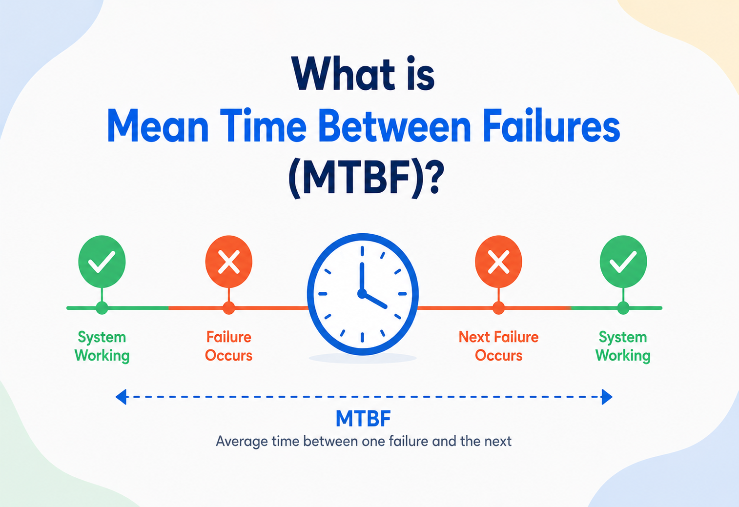
What is Mean Time Between Failures (MTBF)?
A complete, beginner-to-production walk-through of understanding, calculating, and correctly using MTBF — one of the oldest, most widely quoted and most consistently misunderstood numbers in reliability engineering, from hard-drive datasheets and aircraft engines to modern cloud services and microservices.
Introduction & History
Every long-running system, whether a mainframe from 1975 or a Kubernetes cluster from last quarter, eventually meets the same brutal fact: parts break. Mean Time Between Failures — MTBF — is the oldest respectable attempt engineering has to put a number on how often that happens, and how to plan around it.
Imagine you own a car. It breaks down, you get it fixed, and it runs fine for a year. It breaks down again, gets fixed, and runs for another year. If you average this out, you might say “on average, my car goes about a year between breakdowns.” That single sentence — “the average time between one failure and the next” — is the entire idea behind Mean Time Between Failures, usually abbreviated MTBF.
In software and hardware engineering, MTBF is a number, usually measured in hours, that tells you, on average, how long a repairable system runs before it fails. If a fleet of servers has an MTBF of 10,000 hours, it means that — averaged across many failures — a failure happens roughly once every 10,000 hours of operation. It does not mean any single server is guaranteed to run for exactly 10,000 hours; it is a statistical average, much like saying “the average American household has 2.5 children” — no household literally has half a child, but the average is still a useful planning number.
1.1 Where the Term Comes From
MTBF has its roots not in software at all, but in electrical and mechanical engineering, going back to the mid-20th century:
- World War II and early electronics (1940s). As radar, radios, and other electronic equipment became mission-critical for the military, engineers needed a standardised way to describe how often equipment would break down in the field, so commanders could plan spare parts and maintenance schedules.
- MIL-HDBK-217 (US military standard, first published 1965). This handbook formalised methods for predicting the failure rates of electronic components (resistors, capacitors, transistors) and, by extension, the systems built from them — becoming the reference standard for decades of hardware reliability engineering.
- Bell Labs and telecommunications reliability (1950s–1970s). As telephone networks scaled to serve millions of calls, engineers needed rigorous statistical models to guarantee networks would keep working with extremely high uptime — work that heavily influenced how MTBF, alongside related concepts, became standard vocabulary.
- Adoption into computing and, later, cloud / software systems (1980s onward). As computer hardware (hard drives, power supplies, network switches) became critical infrastructure, manufacturers began publishing MTBF ratings for components, and the concept was gradually borrowed by software teams to describe the reliability of entire services, not just physical parts.
Today, MTBF appears everywhere from a hard drive’s datasheet, to a data centre’s generator specifications, to a software team’s internal reliability dashboard tracking how often a service crashes.

Think of MTBF like the “average time between speeding tickets” for a particular driver. If a driver gets one every two years on average, that does not mean they are guaranteed exactly 24 months of clean driving each time — some gaps might be six months, others four years. But over a long enough history, the average settles around two years, and that number is genuinely useful for, say, an insurance company deciding how to price a policy.
Problem & Motivation
Why do engineers need a number like MTBF at all? Why not just say “the system usually works fine”? Because “usually fine” cannot be planned around, budgeted for, or compared between two different designs. MTBF exists to solve several very concrete problems.
You cannot plan maintenance without a number
If you run a data centre with 10,000 hard drives and you do not know their failure rate, you cannot budget for replacement parts, staff a repair team appropriately, or decide when preventive replacement is cheaper than waiting for a failure.
You cannot compare two designs objectively
If Vendor A’s server power supply and Vendor B’s power supply both “seem reliable,” MTBF gives you an actual number to compare — 50,000 hours vs. 80,000 hours — turning a vague impression into a concrete purchasing decision.
You cannot set realistic availability targets
Promising customers “99.99% uptime” requires knowing, statistically, how often your systems fail and how fast you can fix them. MTBF is one half of that equation (the other half being repair time, covered in Section 3).
You cannot detect a system getting worse over time
Without tracking MTBF over time, a service that is slowly degrading (say, crashing every 30 days instead of every 90) can go unnoticed until it becomes a major, customer-visible crisis.
2.1 A Concrete Beginner Example
Suppose a company runs a fleet of 100 identical web servers. Over one year (8,760 hours per server, so 876,000 total server-hours across the fleet), the team observes 20 hardware failures across the fleet. The MTBF is simply the total operating time divided by the number of failures:
Total operating time: 100 servers × 8,760 hours = 876,000 server-hours.
Number of failures: 20.
MTBF = 876,000 ÷ 20 = 43,800 hours (about 5 years) between failures, per server, on average.
This single number lets the operations team estimate: “with 100 servers running continuously, we should expect to handle a failure roughly every 2–3 weeks fleet-wide” — a genuinely actionable staffing and spare-parts planning input.
Without this calculation, the team would only have a vague sense that “servers fail sometimes,” which cannot drive a staffing plan, a budget, or a service-level agreement with customers.
Core Concepts
Let us build the vocabulary carefully, one term at a time, since MTBF is frequently confused with several closely related — but distinct — metrics.
3.1 Failure
What: An event where a system stops performing its required function, according to a clearly defined threshold (e.g., a server crashes, a disk becomes unreadable, an API starts returning errors above some agreed rate).
Why it matters: Without a precise, agreed definition of “failure,” any MTBF number is meaningless — different teams might count things differently, making comparisons invalid.
Analogy: Like a doctor needing a precise definition of “sick” before counting how often a patient gets sick — a sniffle and a hospitalisation should not be counted the same way.
3.2 MTBF (Mean Time Between Failures)
What: The average time a repairable system operates between one failure and the next.
Formula: MTBF = Total Operating Time ÷ Number of Failures
Why it matters: It applies specifically to systems that get repaired and put back into service — a server that crashes, gets rebooted, and keeps running is a great candidate for MTBF. A disposable item that is thrown away after one failure is not (see MTTF below).
3.3 MTTF (Mean Time To Failure)
What: The average time until failure for non-repairable items — things that are replaced, not fixed, once they fail (a light bulb, a single-use battery, sometimes a solid-state drive treated as disposable).
Why it matters: People very commonly misuse “MTBF” when they actually mean “MTTF.” The distinction matters because MTBF assumes a repair-and-return-to-service cycle, while MTTF assumes permanent replacement.

3.4 MTTR (Mean Time To Repair / Restore)
What: The average time it takes to fix a failure once it happens and bring the system back into service.
Why it matters: MTBF alone does not tell you about availability — a system that fails often but is repaired instantly can still have excellent uptime, while a system that fails rarely but takes days to fix can have terrible uptime. You need both numbers together.
3.5 Failure Rate (λ, lambda)
What: The number of failures per unit of time — literally the mathematical reciprocal of MTBF: λ = 1 / MTBF.
Why it matters: Failure rate is what actually feeds into most statistical reliability formulas (like the exponential reliability function in Section 5); MTBF is often just a more human-friendly way of expressing the same underlying number.
3.6 Availability
What: The fraction of time a system is actually up and usable, calculated from both MTBF and MTTR: Availability = MTBF / (MTBF + MTTR).
Why it matters: This is the number that actually matters to end users and to service-level agreements — not MTBF alone. A system can have a mediocre MTBF but excellent availability if MTTR is very small.
Think of MTBF and MTTR like two knobs on the same machine. MTBF is “how often does the machine jam,” and MTTR is “how long does it take someone to un-jam it.” A machine that jams once a day but is fixed in 10 seconds might have better overall uptime than a machine that jams once a month but takes three days to fix. Availability is the number that actually combines both knobs into “how much of the time can I actually use this thing.”
3.7 The Bathtub Curve
What: A classic reliability-engineering model describing how failure rate changes over a system’s lifetime: high failure rate early on (“infant mortality,” defective units failing quickly), a long period of low, roughly constant failure rate (“useful life,” where MTBF applies most cleanly), and rising failure rate again near end-of-life (“wear-out”).
Why it matters: MTBF, as a single average number, is really only meaningful during the flat “useful life” portion of the curve — using it during the infant-mortality or wear-out phases can be seriously misleading.
Architecture & Components of an MTBF Measurement System
Calculating a trustworthy MTBF is not just “divide two numbers” — in a real production environment, it requires a small pipeline of data collection, definition-setting, and calculation, much like any other engineering system.
4.1 Component: Failure Definition / Taxonomy
A documented, agreed set of rules describing exactly what counts as a “failure” for this system — for example, “any hardware fault requiring physical replacement” for a hard-drive fleet, or “any 5-minute period where error rate exceeds 5%” for a software service. Without this, different engineers will count failures inconsistently.
4.2 Component: Operating Time Tracker
A system that tracks exactly how many hours each unit (server, disk, service instance) was actually running and in service — not counting time it was intentionally powered off, in planned maintenance, or not yet deployed.
4.3 Component: Failure Event Log
A structured, timestamped record of every failure, ideally tagged with metadata: which unit failed, what type of failure, and (crucially) whether the unit was subsequently repaired and returned to service (relevant for MTBF) or permanently retired (relevant instead for MTTF).

4.4 Component: MTBF Calculation Engine
The logic (sometimes a simple spreadsheet formula, sometimes a full analytics pipeline at scale) that aggregates total operating time and failure counts, typically segmented by time window, hardware batch, firmware version, or geographic region, to allow meaningful comparisons.
4.5 Component: Reliability Dashboard
A visualisation layer — typically time-series charts — showing MTBF trending over weeks / months / quarters, broken down by relevant dimensions (server model, data centre, software version), so that engineers and leadership can spot deteriorating reliability early.
Large hardware fleets (hyperscale data centres with hundreds of thousands of disks or servers) typically compute MTBF separately per hardware batch and firmware version, because a single bad manufacturing batch or a buggy firmware update can dramatically skew the aggregate number if it is not isolated — a classic example of why segmentation matters enormously once you are operating at scale.
Internal Working — The Math Behind MTBF
Let us go under the hood and understand exactly how MTBF is calculated and what statistical assumptions make it valid (or invalid). The math is intentionally simple; the assumptions behind it are what actually matter.
5.1 The Basic Formula
MTBF = Total Operating Time / Number of FailuresA fleet of 50 network switches runs for 6 months (4,380 hours). During that time, engineers observe 6 failures, and every failed switch was repaired and returned to service (not permanently discarded).
Total operating time = 50 × 4,380 = 219,000 switch-hours.
MTBF = 219,000 ÷ 6 = 36,500 hours (about 4.2 years) between failures, per switch, on average.
5.2 The Exponential Distribution Assumption
MTBF’s simple formula implicitly assumes that failures happen at a constant rate over time — mathematically, that failures follow an exponential distribution. This assumption is what makes MTBF valid specifically during the flat “useful life” portion of the bathtub curve (Section 3), and invalid during infant-mortality or wear-out phases, where the failure rate is actively changing.
Under this assumption, the probability that a system survives without failure past time t is given by the reliability function:
R(t) = e^(-t / MTBF)If MTBF = 10,000 hours, what is the probability a system survives at least 5,000 hours (roughly 7 months) without failing?
R(5000) = e^(−5000/10000) = e^(−0.5) ≈ 0.607, or about a 60.7% chance of no failure in that window.
Notice this is not 50%, even though 5,000 is exactly half of the MTBF — a common intuition mistake. The exponential distribution is not symmetric like a bell curve; it is “memoryless” (explained next).
5.3 The “Memoryless” Property — A Crucial and Counter-intuitive Fact
Because of the exponential distribution assumption, MTBF has a strange but important property: a system that has already been running for 5 years with no failure is, statistically, exactly as likely to fail in the next hour as a system that was just turned on. The system does not “remember” how long it has already survived. This is extremely counter-intuitive (it feels like an old system should be “due” for a failure), but it is mathematically true under the constant-failure-rate assumption — and it is exactly why the bathtub curve’s wear-out phase (where this assumption breaks down) matters so much in real hardware.
This is one of the most common conceptual mistakes with MTBF: treating a high MTBF (say, 1,000,000 hours, which is roughly 114 years) as a guarantee that “this specific unit will individually last 114 years.” It does not mean that at all. A million-hour MTBF simply means that if you had a very large number of these units running simultaneously, on average one failure would occur for every million hours of combined operating time across all of them — it says nothing about any single unit’s actual lifespan, especially given wear-out effects.
5.4 MTBF and Availability Together
As introduced in Section 3, MTBF alone does not determine uptime — you need MTTR too:
Availability = MTBF / (MTBF + MTTR)Two systems both have an MTBF of 1,000 hours.
System A has an MTTR of 1 hour: Availability = 1000 / (1000 + 1) = 99.90%.
System B has an MTTR of 10 hours: Availability = 1000 / (1000 + 10) = 99.01%.
Same MTBF, but System A delivers roughly ten times fewer “nines” of downtime than System B — proving why MTTR (fast detection and repair) is often a more cost-effective investment than chasing an ever-higher MTBF.
5.5 A Small Java Tool to Compute MTBF, MTTR, and Availability
import java.time.Duration;
import java.util.*;

public class ReliabilityCalculator {

    record FailureEvent(Duration timeSinceLastFailure, Duration repairDuration) {}

    private final List<FailureEvent> events = new ArrayList<>();

    public void recordFailure(Duration timeSinceLastFailure, Duration repairDuration) {
        events.add(new FailureEvent(timeSinceLastFailure, repairDuration));
    }

    public Duration meanTimeBetweenFailures() {
        long totalOperatingSeconds = events.stream()
                .mapToLong(e -> e.timeSinceLastFailure().toSeconds())
                .sum();
        return Duration.ofSeconds(totalOperatingSeconds / Math.max(1, events.size()));
    }

    public Duration meanTimeToRepair() {
        long totalRepairSeconds = events.stream()
                .mapToLong(e -> e.repairDuration().toSeconds())
                .sum();
        return Duration.ofSeconds(totalRepairSeconds / Math.max(1, events.size()));
    }

    public double availability() {
        double mtbfSeconds = meanTimeBetweenFailures().toSeconds();
        double mttrSeconds = meanTimeToRepair().toSeconds();
        return mtbfSeconds / (mtbfSeconds + mttrSeconds);
    }

    // Probability the system survives past a given duration without failing,
    // assuming a constant failure rate (exponential distribution).
    public double survivalProbability(Duration t) {
        double mtbfHours = meanTimeBetweenFailures().toSeconds() / 3600.0;
        double tHours   = t.toSeconds() / 3600.0;
        return Math.exp(-tHours / mtbfHours);
    }

    public static void main(String[] args) {
        ReliabilityCalculator calc = new ReliabilityCalculator();
        calc.recordFailure(Duration.ofHours(4200), Duration.ofMinutes(45));
        calc.recordFailure(Duration.ofHours(3900), Duration.ofMinutes(30));
        calc.recordFailure(Duration.ofHours(4500), Duration.ofMinutes(20));

        System.out.println("MTBF: " + calc.meanTimeBetweenFailures().toHours() + " hours");
        System.out.println("MTTR: " + calc.meanTimeToRepair().toMinutes() + " minutes");
        System.out.printf("Availability: %.4f%%%n", calc.availability() * 100);
        System.out.printf("P(no failure in next 1000 hours): %.4f%n",
                calc.survivalProbability(Duration.ofHours(1000)));
    }
}Data Flow & Lifecycle of an MTBF Metric
Let us trace how a single failure event, all the way from occurrence to influencing a design decision, flows through an organisation’s reliability process.
6.1 Stage 1 — Deployment and the Operating-Time Clock Starts
The moment a unit (a server, a disk, a service instance) enters production, its “operating time” clock begins. This clock typically pauses during planned maintenance windows and resumes afterward, since MTBF is meant to reflect unplanned failures, not scheduled downtime.
6.2 Stage 2 — Continuous Monitoring
Automated health checks (heartbeats, disk SMART data, service-level error rates) continuously watch for the failure conditions defined in the failure taxonomy (Section 4).
6.3 Stage 3 — Failure Detection and Logging
When a failure condition is met, it is timestamped and logged with relevant metadata: which unit, what type of failure, and environmental context (temperature, load, recent changes).
6.4 Stage 4 — Repair and Return to Service
For MTBF (as opposed to MTTF) to apply, the failed unit must be repaired and returned to operation — this repair event and its duration feed directly into the MTTR calculation described in Section 5.
6.5 Stage 5 — Aggregation into MTBF
Periodically (often nightly or weekly), a calculation engine aggregates all operating time and failure counts across the fleet (or a relevant segment of it) to compute a fresh MTBF figure.

6.6 Stage 6 — Trend Visualisation
The computed MTBF is charted over time, ideally broken down by dimensions like hardware batch, firmware version, or data centre — a flat or improving trend is good news; a declining trend is an early warning sign.
6.7 Stage 7 — Decision-making
Declining MTBF for a specific batch or component often triggers concrete action: a firmware rollback, a hardware recall, a design change in the next product revision, or adjusted spare-parts inventory and staffing.
Advantages, Disadvantages & Trade-offs
MTBF is a powerful number when handled with care, and a dangerously misleading number when quoted without context. Here is a balanced look at what it gives you, what it hides, and the trade-offs that come with using it.
7.1 Advantages
| Advantage | Why it matters |
|---|---|
| Enables objective comparison | Turns “this seems reliable” into a real number you can compare across vendors, designs, or time periods. |
| Drives maintenance and spares planning | Lets operations teams forecast how many replacement parts and how much repair staffing capacity they will need. |
| Feeds directly into availability calculations | Combined with MTTR, MTBF is a direct input to SLA design and uptime commitments. |
| Widely understood, industry-standard vocabulary | Nearly every hardware datasheet and reliability report uses MTBF, making it a common language across vendors and engineers. |
| Detects reliability regressions early | A dropping MTBF trend is an early warning sign of a manufacturing defect, a bad firmware update, or environmental problems (e.g., overheating). |
7.2 Disadvantages & Common Misuses
| Disadvantage | Why it happens / how to mitigate |
|---|---|
| Frequently misinterpreted as a guarantee | People assume “MTBF = 1,000,000 hours” means their specific unit will individually last that long — it is a fleet-wide statistical average, not an individual promise. |
| Invalid outside the “useful life” phase | Using MTBF during infant-mortality or wear-out phases (Section 3) produces misleading numbers, since the constant-failure-rate assumption breaks down. |
| Sensitive to sample size | A small number of observed failures produces a statistically noisy MTBF estimate — a fleet with only 2 failures observed cannot support a confident million-hour MTBF claim. |
| Ignores failure severity | MTBF treats a minor, quickly-repaired glitch the same as a catastrophic, data-losing failure unless the failure taxonomy explicitly separates them. |
| Vendor-reported MTBF can be optimistic | Manufacturer MTBF figures are sometimes derived from accelerated lab testing or theoretical component models rather than real-world field data, and can differ substantially from observed field MTBF. |
| Says nothing about downtime duration | A high MTBF with a terrible MTTR can still yield poor availability — MTBF must always be read alongside MTTR (Section 5). |
7.3 Key Trade-off: Statistical Confidence vs. Observation Cost
Getting a statistically reliable MTBF estimate requires observing many failures over a long time — but waiting that long is expensive and slow, especially for expensive, low-failure-rate components. This is why accelerated life testing exists: deliberately stressing components (extreme heat, vibration, voltage) to induce failures faster in a lab, then using statistical models to extrapolate back to normal-condition MTBF — trading test time for a modelling assumption that must itself be validated.
7.4 Key Trade-off: Aggregate Simplicity vs. Hidden Variation
A single, blended MTBF number for an entire fleet is simple to communicate and easy to put in a report, but it can quietly average away a serious localised problem. Ten servers failing constantly and ninety servers never failing at all can produce the exact same aggregate MTBF as one hundred servers each failing at a moderate, uniform rate — yet these two scenarios call for completely different engineering responses (investigate one bad batch, versus a general design improvement across the whole fleet). This is precisely why Section 8 emphasises segmentation as a scaling requirement rather than a nice-to-have.
7.5 Key Trade-off: Theoretical Modelling vs. Empirical Field Data
Reliability predictions can come from two very different sources: theoretical component-count models (adding up individually-modelled failure rates for every resistor, capacitor, and chip in a design, following standards descended from military handbooks) or empirical field data (actually watching real units fail in real conditions over time). Theoretical models are available before a single unit has ever been built or deployed, which is valuable for early design decisions, but they rely on assumptions that may not hold in practice. Empirical field data is far more trustworthy but only becomes available after a system has already been deployed for a meaningful length of time — meaning organisations often have to make important early reliability decisions using the less trustworthy theoretical numbers, then correct course once real field data starts arriving.
Performance & Scalability of MTBF Tracking
Just like the postmortem process discussed in companion guides, MTBF tracking has to scale as fleets grow from a handful of servers to tens or hundreds of thousands of units. Let us look at what breaks and how organisations adapt.
8.1 What Breaks at Scale
- Aggregation hides important variation: a single fleet-wide MTBF can mask the fact that one specific hardware batch or firmware version is failing far more often than the rest — the average looks fine while a subset is quietly rotting.
- Data volume: at hyperscale (hundreds of thousands of disks, for example), naive per-unit tracking and recalculation can become a real data-engineering problem, requiring purpose-built time-series pipelines rather than spreadsheets.
- Segment explosion: as you slice MTBF by model, firmware version, data centre, age cohort, and more, the number of segments can explode, and some segments end up with too few failures to be statistically meaningful.
8.2 How Organisations Scale MTBF Tracking
- Automated telemetry pipelines: large-scale operators (cloud providers, hyperscale data centres) build dedicated pipelines that continuously ingest health signals (SMART data for disks, heartbeat data for servers) and compute rolling MTBF automatically, rather than relying on manual failure logging.
- Cohort-based analysis: grouping units by manufacturing batch, deployment date, or firmware version lets teams detect a “bad cohort” quickly, rather than waiting for the aggregate fleet-wide number to visibly degrade.
- Confidence intervals, not just point estimates: mature reliability programmes report MTBF with a statistical confidence interval (e.g., “43,800 hours ± 6,000 hours at 95% confidence”) rather than a single deceptively precise number, especially for smaller sample sizes.
- Predictive / proactive replacement: some organisations (famously large cloud storage providers) use continuously updated MTBF-like models, combined with SMART / health signals, to proactively replace disks predicted to be near failure, before they actually fail and cause data loss.
Large-scale cloud storage operators have published research (based on studying hundreds of thousands of hard drives in production) showing that real-world field MTBF is often significantly different from vendor-published datasheet MTBF — sometimes because vendor figures come from idealised lab conditions, and real data centres introduce additional stress factors like vibration from adjacent drives, temperature variation, and workload patterns the lab testing did not fully capture.
High Availability & Reliability Connection
MTBF is one of the two foundational numbers (alongside MTTR) that underpin virtually every High Availability (HA) design decision in both hardware and software architecture.
9.1 From MTBF to Redundancy Design
If a single component’s MTBF is not high enough to meet an availability target on its own, engineers add redundancy — extra components that can take over if one fails. The combined MTBF of a redundant system is dramatically higher than any single component’s MTBF, because multiple independent components would all have to fail within the same repair window for the overall system to go down.
Suppose a single server has an MTBF of 10,000 hours and an MTTR of 4 hours, giving it about 99.96% availability alone. If you run two independent, redundant servers behind a load balancer (and the system only fails if both fail simultaneously), the combined system’s effective downtime becomes dramatically smaller — this is the mathematical justification behind why redundancy, not just “better” individual components, is usually the most cost-effective way to reach very high availability targets like 99.999% (“five nines”).
9.2 MTBF and Service Level Objectives (SLOs)
Just as a postmortem process (see the companion guide on post-incident reviews) measures MTTR and recurrence trends after the fact, MTBF is the proactive, forward-looking counterpart: reliability engineers use historical MTBF data to predict how many incidents to expect in a given period, and to set realistic SLOs and error budgets rather than picking uptime targets out of thin air.
9.3 Redundancy Patterns and Their MTBF Implications
| Pattern | Description | Effect on effective MTBF |
|---|---|---|
| Active-passive failover | A standby unit takes over when the primary fails | Effective system MTBF rises substantially, limited by failover detection / switch time |
| Active-active load balancing | Multiple units share load simultaneously; one failing reduces capacity but not availability | Individual unit failures become far less user-visible; system-wide failure requires many simultaneous failures |
| N+1 / N+2 redundancy | Extra spare capacity beyond the minimum needed (common in power supplies, cooling systems) | Tolerates one or more simultaneous failures without any service impact |
| Geographic / multi-region redundancy | Entire data centres or cloud regions are duplicated | Protects against correlated failures (e.g., a regional power outage) that redundancy within one building cannot address |
Think of MTBF-driven redundancy like carrying a spare tyre in your car. Any single tyre might have a long MTBF on its own, but a flat tyre is still inevitable eventually. Carrying a spare does not raise any individual tyre’s reliability — it raises the reliability of your trip, because now a single tyre failure does not strand you. High-availability system design applies exactly this logic at a much larger scale.
Security Angle
MTBF is not primarily a security metric, but it intersects with security engineering in several important ways — and the assumptions behind it can quietly break under attacker pressure.
10.1 Security-Relevant Hardware Failures
Physical security devices — badge readers, biometric scanners, hardware security modules (HSMs) that store encryption keys, and network firewalls — all have their own MTBF ratings. A failing HSM or firewall is not just an availability problem; it can create a security gap (e.g., a firewall failing “open” rather than “closed” during a failure could expose an internal network).
10.2 Fail-safe vs. Fail-open Design Decisions
When designing what happens during a failure (which MTBF tells you will eventually occur), security-critical systems must explicitly decide: should the system “fail closed” (deny access, safer but less available) or “fail open” (allow access, more available but riskier)? This decision is directly informed by understanding a component’s expected MTBF and the consequences of failure.

| Approach | Behaviour on failure | When appropriate |
|---|---|---|
| Fail closed / fail secure | Deny access or stop the system entirely when a security-relevant component fails | High-security contexts: a failed authentication service should not silently allow all requests through |
| Fail open | Continue operating, potentially with reduced security, to preserve availability | Physical safety systems, like a fire door unlocking on power failure so people are not trapped |
10.3 Correlated Failures as a Security Risk Multiplier
MTBF calculations typically assume failures are statistically independent. But a coordinated attack (e.g., a distributed denial-of-service attack, or an exploit targeting a shared vulnerability across an entire fleet of identical devices) can cause many “independent” units to fail simultaneously — violating the independence assumption behind MTBF-driven redundancy planning (Section 9) and catching operations teams by surprise if they have not planned for correlated failure modes.
A fleet of thousands of identical IoT devices, each individually rated with an excellent MTBF, can still all fail together within minutes if they share a single software vulnerability that an attacker exploits at scale. MTBF describes random, independent hardware / software wear-related failure — it says nothing about deliberate, correlated, attacker-driven failure, which requires entirely separate security engineering (patching, network segmentation, intrusion detection) to address.
Monitoring, Logging & Metrics
Just as with post-incident reviews, MTBF is only as trustworthy as the telemetry feeding it. Let us look at what good MTBF-supporting observability actually looks like.
11.1 What Needs to Be Measured
| Signal | Purpose | Example source |
|---|---|---|
| Heartbeats / health checks | Detects when a unit stops responding, marking a failure’s start time | Kubernetes liveness probes, hardware BMC heartbeat |
| SMART data (for disks) | Predictive signals (reallocated sectors, read errors) that often precede an outright failure | Disk controller self-monitoring reports |
| Error rate / latency metrics | Defines a software “failure” threshold precisely (e.g., error rate > 5% for 5 minutes) | Prometheus, Datadog, application-level metrics |
| Repair / replacement event logs | Marks exactly when a unit returned to service, closing the failure interval and starting the MTTR clock | Maintenance ticketing systems, deployment logs |
11.2 Building an Accurate Failure Log
Just as a postmortem needs an accurate, agreed timeline (see the companion guide), an MTBF calculation needs an accurate, consistently-defined failure log. This means: precise timestamps (ideally to the second, in UTC), a consistent failure-type taxonomy applied by every team the same way, and a clear distinction between “failure” (unplanned) and “maintenance” (planned, should not count against MTBF).
A data centre operator notices their computed MTBF for a certain server model suddenly drops sharply one quarter. Investigating the failure log reveals that a new ticketing system started auto-logging routine firmware updates as “failures” by mistake, because the servers briefly went offline during the update. After correcting the taxonomy to exclude planned maintenance, the “true” MTBF for unplanned failures returns to its expected historical range — a good illustration of why definitional discipline matters as much as the math itself.
11.3 Dashboards and Alerting on MTBF Trends
Mature reliability programmes do not just compute MTBF once — they track it continuously on dashboards, with alerts configured to fire if MTBF for any tracked segment (a hardware batch, a firmware version, a specific service) drops below a defined threshold, giving engineers an early, proactive warning rather than discovering the problem only after a major outage.
Deployment & Cloud
In cloud environments, MTBF takes on a slightly different flavour, because the underlying physical hardware is abstracted away — but the underlying principles still matter enormously, both for the cloud provider and for the customer building on top of it.
12.1 MTBF from the Cloud Provider’s Perspective
Cloud providers (AWS, Google Cloud, Microsoft Azure) manage enormous fleets of physical hardware, and internally track MTBF at massive scale to plan hardware refresh cycles, negotiate with hardware vendors, and decide which hardware generations to phase out. Their internal MTBF data directly informs the availability guarantees (SLAs) they can responsibly offer to customers.
12.2 MTBF from the Customer’s Perspective
Customers building on cloud infrastructure typically cannot see or influence the underlying hardware’s MTBF directly — instead, they consume the provider’s published availability SLA (e.g., “99.99% monthly uptime for this service tier”) as an abstraction over the provider’s internal MTBF and MTTR numbers, and design their own redundancy (multi-AZ, multi-region) on top of that abstraction.
12.3 Virtual and Software “Failures” in the Cloud
In cloud-native and containerised environments, “failure” often refers less to physical hardware breaking and more to software-level failures: a container crashing, a virtual machine becoming unresponsive, a pod failing its health check. MTBF concepts still apply directly — you can compute the mean time between pod restarts, between virtual machine failures, or between deployment rollbacks, using exactly the same math.
Some cloud-native reliability teams compute an application-level MTBF specifically for container restarts or pod evictions (e.g., “mean time between OOM-kill events for this service”), which is a direct software-engineering analogue of the hardware-world MTBF concept, and is just as useful for capacity planning, resource-limit tuning, and detecting memory leaks before they become customer-visible incidents.
APIs, Microservices & Distributed Systems
In a microservices architecture, the “system” whose MTBF you care about is rarely a single machine — it is often an entire chain of services that must all work together to serve a single user request. This significantly complicates MTBF analysis.
13.1 System-Level MTBF vs. Component-Level MTBF
If a user-facing request depends on five independent microservices, each with its own MTBF, the overall system’s effective MTBF is generally lower than any single component’s MTBF — because the request fails if any dependency fails (assuming no redundancy). This is a classic “series system” reliability calculation:
1 / MTBF_system ≈ 1/MTBF_A + 1/MTBF_B + 1/MTBF_C + ... (for services in series, no redundancy)Five microservices, each individually rated with an MTBF of 50,000 hours, are chained together with no redundancy — a request must pass through all five to succeed.
Combined failure rate ≈ 5 × (1/50,000) = 1/10,000.
Combined system MTBF ≈ 10,000 hours — five times worse than any single service’s individual MTBF, purely because of the chain dependency. This is exactly why architects push hard for redundancy and graceful degradation at every layer of a microservices chain, not just at the “most important” service.
13.2 Graceful Degradation as an MTBF Mitigation Strategy
Rather than treating every dependency failure as a full system failure, well-designed distributed systems degrade gracefully — for example, if a “recommended products” microservice fails, an e-commerce checkout flow can simply omit recommendations rather than failing the entire checkout. This effectively decouples the “failure” of a non-critical dependency from the “failure” of the overall user-facing system, dramatically improving the system’s effective MTBF from the user’s point of view.
13.3 Correlated Failures Across Shared Dependencies
Just as in Section 10’s security discussion, microservices frequently share common underlying dependencies (a shared database, a shared authentication service, a shared cloud region). If that shared dependency fails, it can simultaneously “fail” many otherwise-independent services at once — violating the statistical independence assumption behind simple MTBF combination formulas, and behind naive redundancy math (Section 9) as well.
| Pattern | Effect on system-level MTBF |
|---|---|
| Series dependency chain (no redundancy) | Combined MTBF worse than any single component (as shown above) |
| Redundant / parallel critical paths | Combined MTBF better than any single component (analogous to Section 9’s redundancy discussion) |
| Graceful degradation for non-critical dependencies | Removes non-critical dependency failures from the “system failure” count entirely |
| Shared, non-redundant dependency (e.g., single shared database) | Creates a correlated single point of failure that can invalidate independence assumptions across seemingly separate services |
Design Patterns & Anti-patterns
The habits that make MTBF numbers useful in practice — and the mirror-image mistakes that turn a reassuring dashboard number into false confidence you will regret.

14.1 Good Patterns
| Pattern | Description |
|---|---|
| Segmented MTBF tracking | Computing MTBF separately by hardware batch, firmware version, or service version, rather than one blended fleet-wide number that can hide localised problems. |
| MTBF paired with MTTR and availability | Never reporting MTBF in isolation — always alongside MTTR and the resulting availability figure, since MTBF alone does not determine uptime. |
| Confidence intervals for small sample sizes | Explicitly stating the statistical uncertainty around an MTBF estimate rather than presenting it as a precise, guaranteed figure. |
| Bathtub-curve-aware interpretation | Recognising when a system is in infant-mortality or wear-out phases, where the constant-failure-rate assumption behind MTBF breaks down, and adjusting expectations accordingly. |
| Redundancy informed by real field data | Basing redundancy and failover architecture decisions on actual observed field MTBF, not just optimistic vendor datasheet numbers. |
14.2 Anti-patterns to Avoid
| Anti-pattern | Why it is harmful |
|---|---|
| Treating MTBF as an individual-unit guarantee | A high fleet-wide MTBF says nothing about any single unit’s actual remaining lifespan — a common and costly misreading. |
| Blindly trusting vendor MTBF figures | Vendor numbers are sometimes derived from theoretical models or accelerated lab tests that do not reflect your actual operating environment. |
| Computing MTBF from too few failures | An MTBF calculated from just one or two observed failures carries enormous statistical uncertainty, even though it can be reported as a single, deceptively confident-looking number. |
| Ignoring the independence assumption | Assuming redundant components will fail independently, when in reality they may share a common cause (same power supply, same firmware bug, same data centre) that causes correlated failures. |
| Mixing planned maintenance into failure counts | Inflates apparent failure rates and produces an artificially pessimistic (or, if done inconsistently, artificially optimistic) MTBF. |
| Chasing MTBF while ignoring MTTR | Investing heavily to push MTBF slightly higher while ignoring a slow, manual repair process, when improving MTTR might deliver far better availability for far less cost. |
Best Practices & Common Mistakes
A tighter, more prescriptive playbook — the habits that make MTBF a decision-driving number rather than a decorative one, and the mistakes that keep showing up in incident retros.
15.1 Best Practices
- Define “failure” precisely and consistently, in writing. Every team computing MTBF should apply the exact same definition, or comparisons become meaningless.
- Always report MTBF alongside MTTR and availability. A standalone MTBF number, without repair-time context, tells only half the story that actually matters to users.
- Segment your data. Track MTBF by hardware batch, firmware / software version, and deployment region to catch localised problems the aggregate number would hide.
- Use confidence intervals for small sample sizes. Be honest about statistical uncertainty rather than presenting a single deceptively precise figure.
- Validate the constant-failure-rate assumption. Check where your system sits on the bathtub curve before trusting the exponential-distribution math behind MTBF.
- Exclude planned maintenance from failure counts. Keep “unplanned failure” and “scheduled downtime” as clearly separate categories.
- Cross-check vendor-published MTBF against your own field data. Real operating conditions frequently differ from lab test conditions.
- Watch for correlated failure risks. Do not assume redundant components fail independently if they share a power source, firmware, or other common dependency.
- Trend it over time; do not just snapshot it once. A single MTBF calculation is a point-in-time estimate; the real value comes from watching the trend for early warning signs.
- Tie MTBF data directly to concrete engineering decisions. Redundancy design, spare-parts budgeting, firmware rollback decisions, and SLA-setting should all be traceable back to real MTBF evidence.
15.2 Common Mistakes
- Quoting a manufacturer’s MTBF figure as if it were a guarantee for an individual unit’s lifespan.
- Computing a single blended MTBF across a fleet with wildly different hardware ages, batches, or firmware versions, hiding important variation.
- Forgetting that MTBF applies to repairable systems, and misapplying it to disposable, non-repaired components where MTTF is the correct term.
- Ignoring the bathtub curve and computing MTBF during a fleet’s early “infant mortality” burn-in period, producing an artificially pessimistic number.
- Assuming redundancy always multiplies reliability as the independence math suggests, without checking for shared, correlated failure modes.
- Never revisiting or updating MTBF estimates as more field data accumulates, leaving decisions based on stale or thin initial estimates.
Real-World Industry Examples
Theory becomes concrete when you see how different industries actually apply MTBF. The examples below range from consumer hard drives to aircraft engines to life-critical medical devices — every one of them running the same underlying math, tuned to its own tolerance for failure.
Hard drive manufacturers & public MTBF datasheets
Storage device manufacturers routinely publish MTBF (or the related “Annualised Failure Rate,” AFR) figures for their drives, often in the range of hundreds of thousands to over a million hours. These figures are widely used by data-centre operators for procurement decisions, though experienced operators know to validate them against their own field observations rather than trusting datasheets blindly.
Large-scale cloud storage field-reliability studies
Major cloud storage and backup companies have published widely-read public studies analysing failure rates across populations of well over 100,000 hard drives in real production data centres, broken down by manufacturer and model. These reports are frequently cited across the industry because they provide real-world field MTBF data as a check against vendor-published lab figures, and have influenced procurement decisions industry-wide.
Aerospace & aviation reliability engineering
Aircraft manufacturers and airlines maintain extremely detailed MTBF tracking for every critical component (engines, hydraulic systems, avionics), because component failure rates directly drive maintenance scheduling requirements mandated by aviation safety regulators — a domain where MTBF-style reliability engineering has been rigorously formalised for many decades, predating its adoption in the software industry by a wide margin.
Telecommunications network reliability
Telecom carriers building “five nines” (99.999% availability) phone-switching systems have historically relied on extremely detailed MTBF and MTTR modelling for every hardware component in the call-routing path, since even brief network-wide outages have severe regulatory and financial consequences — this tradition directly influenced the availability engineering practices later adopted by internet and cloud infrastructure companies.
Automotive & industrial equipment
Manufacturers of vehicles and industrial machinery publish MTBF figures for critical components (engines, transmissions, hydraulic pumps) to inform maintenance scheduling and warranty design — a warranty period is, in effect, a business decision made partly by weighing a component’s expected MTBF against the cost of repairs during that period.
Data-centre power & cooling infrastructure
Beyond servers and disks themselves, the physical infrastructure that keeps a data centre running — backup diesel generators, uninterruptible power supplies (UPS), computer-room air conditioning units, and the electrical switchgear connecting them — all carry their own MTBF ratings, and operators design entire tiers of redundancy (the well-known “Tier I through Tier IV” classification) explicitly around combining these components’ MTBF and MTTR figures to hit specific overall facility availability targets, often expressed as an expected number of minutes of downtime per year.
16.1 Medical Device Reliability Engineering
Manufacturers of life-critical medical equipment — ventilators, infusion pumps, pacemakers — are required by regulators in many countries to document detailed reliability analyses, including MTBF-style calculations, as part of the approval process. Because the cost of a failure in this domain can be a human life rather than a business inconvenience, medical device MTBF requirements are typically far more stringent, and are backed by mandatory field-failure reporting requirements that feed back into ongoing safety monitoring long after a device reaches the market.
The number is only as trustworthy as the underlying failure data, and real field conditions (temperature, vibration, workload patterns, power quality) very often produce different results than idealised laboratory testing — which is why organisations with mature reliability programmes always maintain their own field-failure tracking rather than relying solely on manufacturer specifications.
FAQ
Short, direct answers to the questions that come up most often when engineers, product managers or students first grapple with MTBF — and to the questions interviewers most enjoy asking.
Is MTBF the same as MTTF?
No. MTBF applies to repairable systems that are fixed and returned to service after a failure. MTTF (Mean Time To Failure) applies to non-repairable items that are simply replaced once they fail. The two are often confused, but the underlying assumption — repair-and-reuse vs. discard-and-replace — is fundamentally different.
Does a higher MTBF always mean a more reliable system overall?
Not necessarily on its own. A system’s actual availability depends on both MTBF and MTTR together. A system with a slightly lower MTBF but a much faster repair time (low MTTR) can deliver better overall uptime than a system with a higher MTBF but a very slow repair process.
Can MTBF predict when a specific unit will fail?
No. MTBF is a statistical average across a population of units (or across many failure events on one repaired system), not a prediction for any individual unit. Due to the “memoryless” property of the underlying exponential-distribution assumption, a specific unit’s remaining expected lifespan does not decrease just because it has already survived a long time — until it enters the wear-out phase of the bathtub curve, at which point the constant-failure-rate assumption no longer applies anyway.
Why do vendor MTBF numbers sometimes not match real-world experience?
Vendor figures are sometimes derived from theoretical component models, accelerated lab testing, or idealised operating conditions that do not fully capture real-world stress factors like temperature variation, vibration, power quality, and actual workload patterns. This is why organisations with mature reliability practices track their own field MTBF data rather than relying solely on datasheets.
How does MTBF relate to a Service Level Agreement (SLA)?
An SLA’s uptime commitment (e.g., 99.95%) is effectively a promise derived from the provider’s internal MTBF and MTTR data, combined with redundancy design. Understanding the math in Section 5 and Section 9 lets you sanity-check whether a given SLA commitment is realistically achievable given the underlying architecture.
What is a “good” MTBF value?
There is no universal answer — it depends entirely on the component, the industry, and the consequences of failure. A consumer electronics component might have an acceptable MTBF in the tens of thousands of hours, while an aircraft engine component’s required MTBF (and the surrounding redundancy and inspection regime) is many orders of magnitude more demanding, reflecting the far higher cost of failure.
Should software services track MTBF, or is it just a hardware concept?
Modern software and cloud teams absolutely do track MTBF-style metrics — mean time between crashes, mean time between failed health checks, mean time between incidents of a given severity — applying exactly the same underlying math to software failure events as hardware engineers apply to physical component failures.
Summary & Key Takeaways
If you keep only a handful of ideas from this guide, keep these. They are the sentences most likely to protect you from misreading a vendor datasheet, misdesigning a redundancy scheme, or promising an SLA you cannot honestly deliver.
Key Takeaways
- MTBF (Mean Time Between Failures) is the average operating time between one failure and the next for a repairable system, calculated as total operating time divided by number of failures.
- MTBF descends from mid-20th-century military and telecommunications reliability engineering, later adopted broadly across hardware manufacturing and, eventually, software and cloud infrastructure.
- MTBF is often confused with MTTF (for non-repairable items) and must always be interpreted alongside MTTR to understand actual system availability.
- The math behind MTBF assumes a constant failure rate (an exponential distribution), which is only valid during the flat “useful life” portion of the bathtub curve — not during infant-mortality or wear-out phases.
- MTBF is a statistical, fleet-wide average, not an individual-unit guarantee — a common and consequential misinterpretation.
- At scale, MTBF must be segmented (by hardware batch, firmware version, region) to avoid hiding localised reliability problems inside a reassuring-looking aggregate number.
- MTBF directly drives redundancy architecture, high-availability design, spare-parts planning, and realistic SLA-setting — but redundancy math assumes independent failures, which correlated failure modes (shared dependencies, coordinated attacks) can violate.
- In distributed, microservices-based systems, chained dependencies without redundancy can make a system’s effective MTBF worse than any single component’s individual MTBF — a key argument for graceful degradation and redundancy at every layer.
- Trustworthy MTBF numbers require disciplined, consistent failure definitions and accurate telemetry — garbage data in, garbage MTBF out.
- From hard drives and aircraft engines to cloud services and microservices, MTBF remains one of the most foundational — and most widely misunderstood — numbers in reliability engineering, and understanding its assumptions is what separates a genuinely useful metric from a misleading one.
In the end, MTBF is simply the average heartbeat rhythm of a system’s failures — useful for planning, dangerous when mistaken for a promise about any single beat.