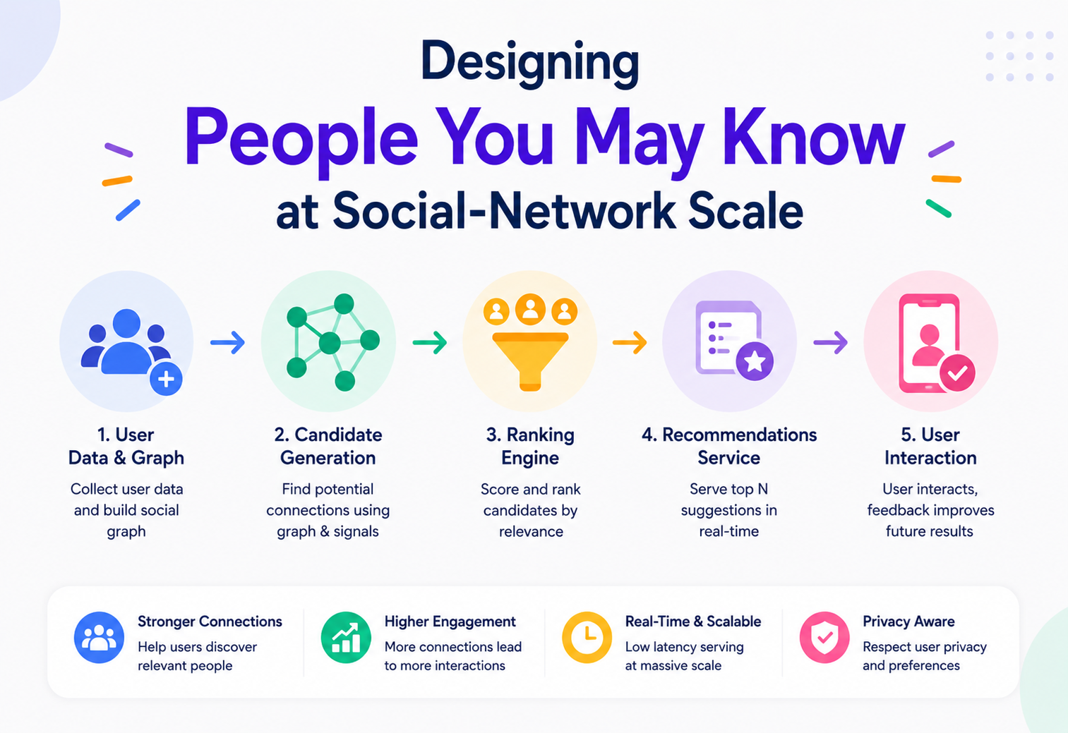
Designing “People You May Know” at Social-Network Scale
A complete, beginner-to-advanced walkthrough of building a personalized friend/connection recommendation system that works for hundreds of millions of users — covering the graph theory, the machine learning, the infrastructure, and the interview questions that come with it.
Introduction & History
Almost every social platform you have ever used — Facebook, LinkedIn, Instagram, Twitter/X, Snapchat — has a small box somewhere in the interface that says something like “People You May Know,” “Suggested for You,” or “People to Follow.” It shows a handful of faces with a name and a small reason underneath, such as “5 mutual friends” or “Works at the same company.” This feature looks tiny, but it is one of the most important growth engines a social network owns.
The idea traces back to the early 2000s. As soon as social graphs became large enough that people could no longer manually find everyone they knew, platforms needed a way to help users rebuild their real-world social circle inside the app. Facebook is widely credited with popularizing “People You May Know” (PYMK) around 2008, using mutual-friend counts as the first, simplest signal. LinkedIn built something similar for professional connections, and over the years both companies (along with Twitter, Instagram, Snapchat, TikTok, and others) evolved these systems from simple graph-counting scripts into massive, multi-stage machine learning pipelines that process billions of graph edges every single day.
Today, a PYMK system is not one algorithm — it is an entire distributed system: graph storage, offline batch jobs, streaming pipelines, machine learning models, caching layers, ranking services, and experimentation frameworks, all working together to answer one deceptively simple question: “Out of the billions of people on this platform, which handful should we show this one user right now?”
A Short Timeline of PYMK
Friendster and early social platforms
The very first web-scale social graphs appear. There is no PYMK yet; users are expected to find their friends themselves. It quickly becomes obvious that manual discovery does not scale beyond a few hundred users.
Facebook popularizes PYMK
Facebook rolls out “People You May Know,” initially powered almost entirely by mutual-friend counts. It becomes a defining growth mechanic and quickly gets copied by every other social platform.
LinkedIn’s professional twist
LinkedIn ships its own PYMK weighted heavily toward shared employer, school, and industry signals rather than personal friend overlap — a first, deliberate demonstration that the same architecture can serve very different products with a different feature mix.
Machine-learned ranking replaces heuristics
Gradient-boosted trees and other supervised learning models replace hand-tuned mutual-friend ordering. Suggestion quality jumps noticeably, and A/B testing frameworks become standard for shipping model changes.
Graph embeddings and GNNs
Node2vec, then Graph Neural Networks, let users be represented as dense vectors that capture structural similarity. Candidate generation shifts from purely explicit graph traversal to include approximate nearest-neighbor search in vector space.
Real-time freshness and privacy discipline
Streaming layers make suggestions react to recent behavior within minutes, and privacy regulation (GDPR-style) reshapes how relationship and contact data can be collected, retained, and deleted — making the block/opt-out filter a mandatory, non-bypassable last step.
Imagine you move to a new city and join a local community center. The receptionist doesn’t just hand you a random list of the 10,000 members. Instead, she thinks: “You mentioned you know Priya — Priya is close friends with Arjun and Meena, so you’ll probably like meeting them too. Also, you both signed up for the same pottery class.” That mental matching — using existing relationships plus shared context to introduce you to the right few people — is exactly what a PYMK system automates, except it does this matching for hundreds of millions of “new members” every day, in milliseconds, using computers instead of a receptionist’s memory.
“Why is PYMK considered a hard system design problem instead of a simple database query?” A strong answer touches on three things: the search space is enormous (the “friend of a friend” graph explodes combinatorially), the ranking needs personalization at massive scale, and the system must run continuously and cheaply for billions of users while staying fresh as the graph keeps changing every second.
1.1 Why This Is a Great System Design Interview Topic
PYMK shows up constantly in system design interviews for a good reason: it touches almost every major theme that interviewers care about in one relatively self-contained problem. It requires graph thinking (how do you represent and traverse a massive relationship graph efficiently), distributed systems thinking (how do you shard, replicate, and keep data fresh across thousands of machines), machine learning systems thinking (how do you go from raw signals to a trained ranking model, and keep training and serving consistent), and product/privacy thinking (how do you balance showing genuinely useful suggestions against very real privacy risks). Very few interview topics let you demonstrate breadth across all of these areas in a single 45-minute conversation, which is exactly why it remains a favorite prompt at companies building any kind of social or networked product.

1.2 Roadmap for This Tutorial
We’ll build up the system in the same order most strong interview answers do: first pin down the problem precisely (Chapter 2), then sketch the high-level architecture (Chapter 3), then zoom into how each piece actually works internally (Chapters 4 through 6), review the trade-offs (Chapter 7), and finally harden the design against the realities of running at scale — performance, reliability, security, observability, deployment, and storage (Chapters 8 through 14) — before closing with patterns, common pitfalls, industry examples, and a summary you can use as a quick-reference cheat sheet (Chapters 15 through 19).
Problem & Motivation
Let’s define the problem precisely before designing anything. What is PYMK supposed to accomplish, why do naive approaches fail, and what must the system guarantee?
2.1 The Business Problem
A social network’s value comes from its network effect — the platform becomes more useful as more of a user’s real-world connections join and stay active. New users who fail to connect with people they know within the first few sessions are far more likely to churn (stop using the app). PYMK exists to solve exactly this: quickly and accurately rebuild a user’s real-world social graph inside the product, which increases engagement, retention, and ultimately the size and health of the whole network.
2.2 The Technical Problem
Formally, for every user u in a graph with hundreds of millions or billions of nodes, we want to produce a ranked list of the top K (say, 10–50) other users who are not already connected to u, ordered by the probability that u will want to connect with them if shown. This must happen:
- At the scale of the entire user base (hundreds of millions to billions of nodes, tens of billions of edges).
- Fast enough to render in a mobile app feed — typically under 100–200 milliseconds for the “read path.”
- Fresh enough to reflect graph changes from the last few minutes to few hours (a user just added 5 new friends; recommendations should adapt).
- Personalized — no two users should generally see the same list.
- Respectful of privacy settings, blocks, and platform policy (never suggest someone who blocked you, or violate a “do not suggest me” preference).
2.3 Why Naive Approaches Fail
The obvious first idea is: “recommend friends-of-friends, ranked by number of mutual connections.” This is a reasonable starting signal, but it breaks down at scale for several reasons, which we’ll unpack throughout this tutorial:
Live friends-of-friends per request
A popular user can have thousands of friends; a 2-hop traversal can touch millions of nodes. Doing this synchronously for every page load is far too slow and too expensive to run at billions of requests/day.
Only mutual-friend count as ranking
Ignores dozens of other useful signals (shared workplace, shared school, contact book matches, co-location, shared groups) and produces generic, sometimes wrong or awkward suggestions.
Recompute from scratch every time
With hundreds of millions of users this becomes a batch job that could take days, making results stale by the time they are shown.
The real solution, which we will build up piece by piece, separates the problem into an offline/near-real-time candidate generation stage (find a manageable set of plausible people, maybe a few hundred, out of billions) and an online ranking stage (score and order that small set using a machine learning model, in milliseconds).
2.4 Functional Requirements
Before drawing any boxes and arrows, it helps to write down exactly what the system must do:
- Given a user, return a ranked list of up to
Ksuggested people, each with a human-readable “reason” (mutual friends, same workplace, and so on). - Never suggest someone who is already connected to the user, someone who has blocked or been blocked by the user, or someone the user has explicitly asked not to be shown.
- Allow the suggestion list to change over time as the underlying graph and user behavior change — a person you just connected with should disappear from the list quickly, and a brand new mutual connection should be able to surface a new suggestion.
- Support feedback actions (dismiss, “not interested,” connect) that influence future suggestions for that user.
- Work uniformly whether the requesting user has 5 connections (a brand-new user) or 5,000 connections (a power user), which is a very different traversal problem in each case.
2.5 Non-Functional Requirements
Read latency
p99 under ~150–200 ms. The suggestion box renders inside a mobile feed; users notice and abandon slow-loading UI.
Availability
99.9%+ for the read path. PYMK is a supporting feature, but an outage still degrades experience and growth metrics.
Freshness
Minutes to a few hours. Recommendations that ignore very recent graph changes feel disconnected from reality.
Throughput
Hundreds of millions of requests/day, with sharp peaks during regional “prime time” hours. Must handle steady-state and diurnal spikes without manual intervention.
Scalability
Linear-ish scaling with user base growth. The architecture should not need a redesign every time the user base doubles.
Consistency model
Eventual consistency is acceptable. Strict strong consistency is not needed and would be far more expensive to guarantee at this scale.
A very common opener is: “Let’s design a ‘People You May Know’ feature — where do you start?” The strongest candidates do not jump straight to boxes and arrows. They spend the first few minutes clarifying functional requirements (what exactly gets shown, what “reasons” are needed, how feedback is used) and non-functional requirements (scale, latency budget, freshness expectations, consistency tolerance) before sketching any architecture. This signals structured thinking and avoids designing the wrong system.
Expect: “How would you estimate the scale of this system?” Practice back-of-the-envelope math: 500 million daily active users, average 300 friends each, meaning roughly 150 billion edges. If each user’s PYMK request needs to explore 2 hops of a graph where each hop can multiply the fan-out by 300x, unbounded traversal is clearly infeasible — this justifies precomputing candidates offline.
Architecture & Components
A production PYMK system is generally organized into three broad layers: offline/batch (heavy graph computation done periodically), near-real-time/streaming (keeps things fresh between batch runs), and online serving (answers the actual app request in milliseconds).
Figure 1 — PYMK end-to-end architecture: raw signals feed offline batch and near-real-time layers, which populate a candidate store the online serving layer consumes within a strict latency budget.
How to read this diagram: Data enters from the left (raw graph edges, contact uploads, profile fields, activity events). The offline layer periodically (say, every 6–24 hours) crunches the entire graph to generate a broad candidate list per user — this is the expensive part done in bulk, using distributed processing frameworks like Apache Spark or Flink. The streaming layer patches those candidate lists in near-real-time so that very recent actions (like accepting a new friend request) are reflected quickly without waiting for the next full batch run. Finally, the online serving layer is what actually answers the mobile app’s request: it reads precomputed candidates from a fast key-value store, re-ranks them using a lightweight ML model, applies privacy/policy filters, and returns the final list — all within a strict latency budget.
3.1 Core Components Explained
Graph Storage
Stores the social graph as an adjacency structure — who is connected to whom. Distributed graph DB, or a sharded key-value store storing adjacency lists (e.g., a custom store on top of RocksDB, or a graph database).
Candidate Generation Jobs
For each user, produce a bounded set (hundreds) of plausible connections using multiple strategies. Spark/Flink jobs running graph traversal and embedding similarity search.
Feature Store
Stores precomputed features per user and per user-pair used by the ranking model. Feast-like feature store systems, key-value store.
Embedding Service
Learns dense vector representations of users from the graph, used for similarity-based candidate generation. GNN training pipeline, ANN index (HNSW).
Ranking Model Service
Scores each candidate for a given user with a probability of “will connect if shown.” Gradient-boosted trees or deep learning served via a low-latency inference service.
Filter / Policy Service
Removes blocked users, respects privacy settings, applies business rules (e.g., don’t over-suggest the same person repeatedly). Rule engine, in-process filters.
PYMK API
Front door that assembles the final response for the client. REST/gRPC microservice behind an API gateway.
“Why split candidate generation and ranking into two stages instead of one model that does everything?” This is a classic recommendation-system interview question. The answer: candidate generation must be cheap enough to consider millions of possible people, so it uses simple, fast heuristics or approximate nearest-neighbor search; ranking is expensive (it can use a rich model with many features) but only needs to run on a few hundred already-filtered candidates. This “funnel” design (broad-and-cheap, then narrow-and-precise) is standard across nearly all large-scale recommender systems — search, ads, feeds, and PYMK included.
3.2 Graph Partitioning Strategies
How the graph is split across machines has a large effect on how efficient the offline batch computation is, since graph algorithms are fundamentally about following edges between nodes — and following an edge that crosses machine boundaries is far more expensive (it requires network communication) than following an edge that stays within the same machine.
Hash-based partitioning
Assign each user to a shard based on a hash of their user ID. Very simple and gives an even load distribution, but ignores graph structure, so many edges cross shard boundaries, increasing cross-machine communication during traversal.
Community-aware partitioning
Use a graph-partitioning algorithm that keeps densely-connected clusters of users (like real-world friend groups) together on the same shard. Reduces cross-shard edges for typical social graphs, but the partitioning itself is expensive and needs periodic rebalancing.
Edge-cut vs. vertex-cut
Edge-cut assigns whole vertices to shards (crossing edges are the “cut”); vertex-cut splits high-degree vertices’ edges across multiple shards. Vertex-cut specifically helps with the “celebrity problem” described later in Chapter 8, since it avoids concentrating an extremely high-degree node’s entire edge list on one shard.
3.3 Separation of Concerns Between Layers
A useful mental model for this architecture is that each layer optimizes for a different variable. The offline batch layer optimizes for thoroughness and cost-efficiency, since it has hours to work with and can use the cheapest available compute. The streaming layer optimizes for freshness, accepting a simpler, less thorough computation in exchange for reacting within minutes. The online serving layer optimizes purely for latency, deliberately pushing as much work as possible into the other two layers so that the request-time computation is as close to “just a few fast lookups plus one small model inference call” as possible. Keeping this separation clean — resisting the temptation to do “just one more computation” inline in the serving path — is one of the most important architectural disciplines in a system like this.
Internal Working — Candidate Generation & Ranking
The two-stage funnel in detail: how a bounded set of plausible candidates is generated, and how a machine-learned ranker turns that set into an ordered, personalized list.
4.1 Candidate Generation Strategies
No single method finds every good suggestion, so real systems combine several candidate-generation strategies and merge the results (this is often called a “multi-source” or “multi-channel” candidate generation approach).
Friends-of-friends (2-hop traversal)
For user u, look at u’s direct connections, then their connections (2-hop neighbors), and count how many paths lead to each candidate. Computed offline using distributed graph processing, not live per-request.
Contact book matching
If a user uploaded their phone contacts (with consent), match phone numbers/emails against other users to suggest people who are already in their real-world address book.
Co-location / co-occurrence
People who attended the same events, joined the same groups, work at the same company, or studied at the same school.
Embedding similarity
Train a model (often a GNN, or simpler techniques like node2vec) that turns every user into a dense vector such that “similar” users end up close together in vector space. Use approximate nearest-neighbor search to find candidates close to the user’s vector.
Reciprocal signals
People who have already viewed or searched for the user’s profile (if privacy settings allow using this signal).
Figure 2 — Multi-source candidate generation feeds a bounded pool into the ranking stage.
4.2 The Friends-of-Friends Graph Traversal, in Detail
This is the foundational signal, so it deserves a close look. Consider a small example: Alice is connected to Bob and Carol. Bob is connected to Dave. Carol is also connected to Dave. Dave is not connected to Alice. From Alice’s perspective, Dave is a strong candidate because there are two independent paths (through Bob and through Carol) connecting Alice to Dave — this is the “2 mutual friends” signal.
Computing this for every user across the whole graph naively (a full breadth-first search from every node) is far too slow — this is a classic example of why we cannot run graph algorithms live, per-request, in a system with billions of edges. Instead, this is computed as a distributed batch job, often using a “triangle counting” or “two-hop neighborhood” style computation across a cluster, where the graph is partitioned across many machines and each machine works on its slice in parallel.
Beginner Example
Think of it as: “for every pair of people who share at least one mutual friend, and who are not already friends, count how many mutual friends they share, then keep the top pairs.” On a whiteboard with 10 people, you could do this by hand in a minute. At 500 million people, you need a distributed system that shards the graph across thousands of machines and runs this counting job in parallel, usually finishing in a few hours.
Production Example
Companies operating at this scale typically run this kind of computation as a nightly or multiple-times-per-day Spark/Flink job over a partitioned copy of the graph stored in a distributed file system (like HDFS or cloud object storage), writing the resulting candidate lists into a fast key-value store that the online service can read with single-digit-millisecond latency.

4.3 Sample Code — Bounded 2-Hop Traversal (Java)
The following simplified Java snippet shows the core idea of a bounded, degree-capped 2-hop traversal, similar to what a batch job would compute per user (in reality this runs distributed across a cluster, not on a single machine, but the logic is the same).
public class MutualFriendCandidateFinder {

    // adjacency: userId -> set of friend userIds
    private final Map<Long, Set<Long>> adjacency;
    private static final int MAX_DEGREE_TO_EXPAND = 2000; // cap high-degree hubs

    public MutualFriendCandidateFinder(Map<Long, Set<Long>> adjacency) {
        this.adjacency = adjacency;
    }

    // returns candidateId -> mutualFriendCount for the given user
    public Map<Long, Integer> findCandidates(long userId) {
        Set<Long> directFriends = adjacency.getOrDefault(userId, Collections.emptySet());
        Map<Long, Integer> mutualCounts = new HashMap<>();

        for (Long friendId : directFriends) {
            Set<Long> friendOfFriend = adjacency.getOrDefault(friendId, Collections.emptySet());

            // cap traversal fan-out for extremely high-degree "hub" nodes
            if (friendOfFriend.size() > MAX_DEGREE_TO_EXPAND) {
                continue;
            }

            for (Long candidate : friendOfFriend) {
                if (candidate.equals(userId) || directFriends.contains(candidate)) {
                    continue; // skip self and existing friends
                }
                mutualCounts.merge(candidate, 1, Integer::sum);
            }
        }
        return mutualCounts;
    }
}
Notice the MAX_DEGREE_TO_EXPAND cap — this is important in real systems. Some accounts (celebrities, brand pages) have millions of connections; expanding through them would be extremely expensive and would produce low-quality, generic candidates. Capping fan-out through high-degree “hub” nodes is a common, practical optimization.
“How would you handle a celebrity account with 50 million followers in your friends-of-friends computation?” The expected answer is exactly the degree-capping technique above, sometimes combined with sampling (randomly sample a subset of a hub’s connections instead of using all of them) so the computation stays bounded regardless of how large a single node’s degree is.
4.4 Ranking: Turning Candidates into a Final Ordered List
Once we have a bounded candidate set (typically a few hundred people per user), the online ranking stage scores each one using a machine learning model trained to predict the probability that the user will send a connection request (or accept one) if shown that suggestion. Typical input features include:
- Number of mutual connections, and their “quality” (mutual friends who are themselves close friends count more than distant acquaintances)
- Profile similarity: same city, same employer, same school, overlapping interests
- Interaction history: has the user viewed this candidate’s profile recently, exchanged messages, or been suggested before and ignored them
- Embedding similarity score from the graph neural network
- Recency signals: the candidate joined recently, or the mutual connection was made recently
These features feed into a model — historically gradient-boosted decision trees (like XGBoost/LightGBM) were very common for this because they are fast, interpretable, and work well on structured/tabular features; increasingly, deep learning ranking models (including two-tower neural networks) are used, especially when combined with learned embeddings.
Candidate generation is like a librarian quickly pulling 300 books off the shelves that might match your taste, based on broad categories. Ranking is like a knowledgeable friend who then reads the back cover of each of those 300 books and hands you the best 10, in order, based on everything they know about your specific preferences.
4.5 Feature Engineering in Detail
The quality of the ranking model depends heavily on the features it is given, arguably even more than on the specific model architecture chosen. Features generally fall into a few buckets:
Structural features
Mutual connection count, weighted mutual count (weighting close mutuals higher), shortest path length, common neighborhood overlap ratio (Jaccard similarity of the two users’ connection sets).
Similarity features
Same city/region, same employer, same school, same industry, age similarity, overlapping interests or groups.
Interaction features
Has candidate’s profile been viewed recently, have they exchanged messages, appeared together in the same photo or post, search history overlap.
Embedding-based features
Cosine similarity between the two users’ learned graph embedding vectors.
Temporal / recency features
How recently did the candidate join, how recently was the mutual connection formed, how long ago was this pair last shown as a suggestion.
Popularity / quality features
Candidate’s own connection count (extremely high-degree accounts are sometimes down-weighted, since indiscriminately connecting with them is a weaker signal of a meaningful real-world relationship).
A subtlety worth understanding: features must be computed consistently between training time (using historical data) and serving time (using live data), otherwise the model will behave unpredictably in production even though it looked accurate during training — this mismatch is known as “training-serving skew,” and is one of the most common real-world bugs in recommendation systems. This is precisely why a dedicated feature store (Chapter 3.1) is used: it acts as a single source of truth for how each feature is computed, shared by both the offline training pipeline and the online serving path.
4.6 How the Ranking Model Is Trained
The model is trained as a supervised learning problem. Historical logs of past suggestions — which candidates were shown to which users, and whether the user subsequently sent or accepted a connection request — become the labeled training data (a suggestion the user acted on is a positive example; one they ignored is a negative example). Because the number of “ignored” suggestions vastly outnumbers “acted on” suggestions, techniques like negative sampling or class-weighting are used so the model doesn’t simply learn to predict “no” for everything.
The trained model is validated offline against a held-out slice of historical data (checking metrics like AUC — area under the ROC curve — which measures how well the model ranks positive examples above negative ones), and only promoted to production after passing these offline checks and, subsequently, a live online experiment (see Chapter 12 on canary/shadow deployment).
4.7 Sample Code — Simplified Feature Vector Assembly (Java)
public class CandidateFeatureBuilder {

    private final FeatureStoreClient featureStore;

    public CandidateFeatureBuilder(FeatureStoreClient featureStore) {
        this.featureStore = featureStore;
    }

    public FeatureVector build(long userId, long candidateId) {
        int     mutualCount              = featureStore.getMutualConnectionCount(userId, candidateId);
        double  embeddingSimilarity      = featureStore.getEmbeddingCosineSimilarity(userId, candidateId);
        boolean sameEmployer             = featureStore.isSameEmployer(userId, candidateId);
        boolean sameSchool               = featureStore.isSameSchool(userId, candidateId);
        long    daysSinceCandidateJoined = featureStore.getDaysSinceJoined(candidateId);
        int     candidateDegree          = featureStore.getConnectionCount(candidateId);

        return FeatureVector.builder()
                .mutualConnectionCount(mutualCount)
                .embeddingCosineSimilarity(embeddingSimilarity)
                .sameEmployer(sameEmployer)
                .sameSchool(sameSchool)
                .daysSinceCandidateJoined(daysSinceCandidateJoined)
                .candidateDegree(candidateDegree)
                .build();
    }
}“How would you handle the ‘cold start’ problem for a brand new user with zero connections?” Expect a discussion of fallback strategies: for users with no graph signal yet, lean on non-graph signals such as contact-book matching, same school/employer, or geographic proximity, and consider surfacing popular or highly-connected “hub” accounts relevant to the user’s stated interests as an interim strategy until the user builds enough graph structure for the standard pipeline to work well.
4.8 Diversity and the “Filter Bubble” Problem
Pure score-maximization in the ranking stage has a subtle failure mode: if you simply sort every candidate by predicted score and take the top K, you can end up showing a user ten near-duplicate suggestions — for instance, ten different coworkers from the same small team, when the user might actually be more interested in seeing a broader mix of coworkers, former classmates, and friends-of-friends. To address this, production ranking pipelines usually apply a diversity or re-ranking pass after the raw model scores are computed, using techniques such as capping how many top results can share the same “source strategy” or the same underlying mutual connection, so the final list feels varied and useful rather than narrowly repetitive.
4.9 Generating Human-Readable Reasons
The short “reason” text shown under each suggestion (like “5 mutual connections” or “Works at the same company”) is not just a cosmetic detail — research and product experience across social platforms consistently show that a suggestion accompanied by a clear, truthful reason is far more likely to be acted on than one shown with no context at all, since it gives the user an immediate, low-effort way to judge relevance. Generating this reason is typically done by picking the single strongest contributing feature for that specific candidate (whichever feature had the largest positive influence on the model’s score) and mapping it to a pre-written, human-friendly template, rather than trying to explain the full, more complex combination of signals the ranking model actually used internally.
Data Flow & Lifecycle
Let’s trace a request end-to-end, followed by how the underlying data refreshes over time.
Figure 3 — End-to-end read path for a PYMK request, from mobile app to filtered top-K response.
5.1 Lifecycle of a Suggestion
Generation
The offline batch pipeline computes broad candidate pools every few hours using the strategies from Chapter 4.
Freshening
A streaming layer listens to real-time events (new connections, profile edits, blocks) via a message queue like Kafka, and patches the precomputed candidate store incrementally so results don’t feel stale for hours.
Caching
When a user opens the app, the online service first checks a fast in-memory cache (like Redis) before falling back to the underlying store, to keep latency low for repeat requests.
Ranking
Candidates are scored by the ranking model using the freshest available features.
Filtering
Business rules and privacy checks strip out anyone who should never be shown (blocked users, people who opted out, duplicate recent suggestions).
Feedback loop
Whether the user clicks, ignores, or dismisses a suggestion is logged as a training signal for the next model training cycle — this closes the loop and lets the system keep improving.
“How do you keep recommendations fresh if the heavy computation only runs every few hours?” Expect the interviewer to be checking whether you know the batch-plus-streaming (“Lambda architecture”-style) pattern: heavy, accurate computation offline, lightweight incremental patches online, so the system is both eventually thorough and always reasonably fresh.
5.2 What the Streaming Layer Actually Patches
It’s worth being concrete about what “patching” means in practice, since the streaming layer does not attempt to redo the full candidate-generation computation — that stays the job of the batch layer. Instead, it handles a small set of high-value, cheap-to-apply updates:
- Removing stale candidates: if user A and user B just became connected, B should be removed from A’s candidate list (and vice versa) immediately, rather than waiting for the next batch run — showing someone a suggestion to connect with someone they’re already connected to looks obviously broken.
- Applying new exclusions: if user A blocks user B, that exclusion must propagate to the candidate store within seconds, not hours, given the privacy sensitivity involved.
- Light-touch promotion of very strong new signals: if two users who weren’t previously connected suddenly share a brand new, strong mutual connection (for example, a mutual friend they just both connected with), a lightweight incremental score bump can be applied without a full recomputation.
Anything requiring a broader recomputation — like fully re-deriving someone’s entire candidate pool from scratch — is deliberately left to the next batch cycle, since attempting to do that work incrementally, for every single event, would essentially mean re-implementing the batch pipeline’s logic in a much more complex, per-event streaming form, for relatively little added benefit.
Algorithms, Data Structures & Capacity Estimation
The specific algorithms and data structures that make the funnel work at scale — plus a back-of-the-envelope walkthrough of the sizing numbers that justify every downstream design choice.
6.1 Graph Representation
At this scale, the graph cannot live in memory on a single machine. It is partitioned (“sharded”) across many machines, typically by user ID ranges or using a graph-partitioning algorithm that tries to keep highly-connected clusters of users together on the same shard to minimize cross-machine traffic during traversal. Each shard stores an adjacency list: for each user, the list of user IDs they are connected to.
6.2 Approximate Nearest Neighbor (ANN) Search
Once users are represented as dense vectors (embeddings) via a graph neural network or similar technique, finding “similar” users becomes a nearest-neighbor search problem in high-dimensional space. Doing this exactly (comparing a user’s vector against every other user’s vector) is far too slow at hundreds of millions of vectors. Instead, systems use approximate nearest neighbor structures such as HNSW (Hierarchical Navigable Small World graphs) or IVF (Inverted File Index) that trade a small amount of accuracy for enormous speed gains — typically finding “good enough” nearest neighbors in milliseconds instead of seconds.
6.3 Union-Find / Connected Components for Community Detection
Some candidate-generation strategies benefit from knowing which “community” or cluster a user belongs to (e.g., a friend group, a school cohort). Union-Find (Disjoint Set Union) is a classic data structure used in distributed graph processing to efficiently group nodes into connected components, which can be used as an additional candidate-generation signal (“suggest other members of this densely-connected friend cluster”).
6.4 Bloom Filters for Fast “Already Connected” Checks
A very practical optimization: before doing expensive candidate scoring, systems often use a Bloom filter (a compact, probabilistic data structure) to quickly check “is this candidate already a connection, or already dismissed by the user?” A Bloom filter can answer this in constant time with very low memory usage, at the cost of a small false-positive rate (which is acceptable here, since worst case we just skip a few valid candidates).

6.5 Consistent Hashing for Sharding the Cache and Store
To distribute candidate lists and cache entries evenly across many machines — and to avoid a massive reshuffle whenever a machine is added or removed — consistent hashing is used, just as in most large-scale distributed caching systems.
6.6 Consensus for Metadata, Not for Every Edge
It’s a common misconception that a system like this needs a strong consensus protocol (like Raft or Paxos) guarding every single graph edge write. In practice, consensus algorithms are reserved for a much smaller, more critical set of metadata — for example, agreeing on shard ownership assignments, coordinating leader election within a storage cluster, or managing configuration changes to the partitioning scheme. The actual high-volume graph edge writes and candidate list updates use the simpler, higher-throughput eventual-consistency replication model described in Chapter 8, because requiring full consensus for every one of billions of daily graph mutations would be prohibitively slow and would not meaningfully improve the user-facing product, given that eventual consistency is already an acceptable trade-off here.
“Why not use an exact nearest-neighbor search since accuracy matters for good recommendations?” Good answer: exact search is O(n) per query against every vector, which at hundreds of millions of users is computationally infeasible within a latency budget of milliseconds. Approximate methods like HNSW give recall in the high 90s% range while being orders of magnitude faster, which is the right trade-off for a recommendation system (unlike, say, a fraud detection system where exactness might matter more).
6.7 How Graph Embeddings Are Actually Learned
It’s worth spending a moment on how a user “becomes” a vector, since this is one of the more conceptually tricky parts of the system for newcomers. The general idea, shared by techniques like node2vec and modern Graph Neural Networks (GNNs), is: a user’s vector should be learned such that users who are structurally close in the graph end up close together in vector space, and users who are structurally distant end up far apart.
One classical approach, node2vec, works by simulating many random walks starting from each node in the graph (a “random walk” means repeatedly hopping to a randomly chosen neighbor). This turns the graph into something that looks like a collection of “sentences,” where each “word” is a user ID and each “sentence” is a random walk path. These synthetic sentences are then fed into a word-embedding-style model (conceptually similar to Word2Vec, originally built for natural language) which learns vectors such that users appearing near each other in these random-walk sentences end up with similar vectors.
Modern systems increasingly use Graph Neural Networks instead, which improve on this by also incorporating each user’s own features (not just graph position) — for example, profile attributes, activity level, and the features of their neighbors — through a process called “message passing,” where each node repeatedly aggregates information from its neighbors across several rounds (or “layers”) to build a richer representation. This lets the model learn things like “users are similar not only because they are graph-close, but because their neighborhoods share similar characteristics.”
Think of node2vec’s random walks like this: if you repeatedly wander around a city starting from your house — sometimes turning left, sometimes right, always following streets — the places you end up visiting most often reveal something about your neighborhood’s structure. If two houses tend to appear in each other’s wandering paths a lot, they are probably close together or well-connected by roads. Embedding models do the same thing mathematically: they learn a “map” (the vector space) where frequently co-visited nodes end up placed near each other.
6.8 Capacity Estimation Walkthrough
Interviewers often want to see you reason quantitatively about scale, not just describe components. Here is a representative walkthrough:
Raw graph edges
~16 bytes per edge (two 8-byte user IDs) in an adjacency-list representation with some overhead. 75 billion edges ≈ a few TB just for the edge list before replication — within reach of a sharded cluster, too large for a single machine.
Candidate store size
500M users × ~300 precomputed candidates × ~20 bytes per entry (ID + score + short reason code) ≈ ~3 TB — easily shardable, not something to fully replicate across dozens of regions without a plan.
Read QPS (average)
200M DAU × 2 reads / day ≈ 400M reads / day ≈ ~4,600 req/s average.
Read QPS (peak)
3–5× average during regional prime-time ≈ 15,000–25,000 req/s at peak. Serving layer must be sized for this, not the average.
None of these numbers need to be exact in an interview — the point is to demonstrate that you can translate a vague scale (“social-network scale”) into concrete numbers that justify specific design decisions, like why a single-machine graph database is not viable and why sharding and caching are necessary rather than optional.
Advantages, Disadvantages & Trade-offs
Every choice this design makes gives up something in exchange for something else. Reasoning through these trade-offs explicitly is often what separates a strong system design answer from an average one.
Offline batch candidate generation
Pros: Can afford expensive, thorough graph computation; scales cheaply with parallelism.
Cons: Results can be stale by several hours until the next run, or until streaming patches catch up.
Two-stage funnel (generate then rank)
Pros: Keeps expensive ranking model limited to a small candidate set, controlling cost and latency.
Cons: If candidate generation misses a good match entirely, ranking never gets a chance to surface it (“recall ceiling”).
Approximate nearest neighbor search
Pros: Massive speed and memory savings at scale.
Cons: Slight loss of accuracy compared to exact search; requires careful index tuning.
Heavy caching of candidate lists
Pros: Very low read latency, reduced load on backing stores.
Cons: Risk of showing stale suggestions if cache invalidation lags behind graph changes.
Multi-channel candidate generation
Pros: Higher quality and diversity of suggestions.
Cons: More engineering complexity, more infrastructure to maintain and monitor.
Community-aware graph partitioning
Pros: Fewer expensive cross-shard edge traversals during batch computation.
Cons: Rebalancing partitions as the graph evolves is itself a non-trivial, periodically recurring cost.
Eventual consistency for graph updates
Pros: Much higher availability and lower write-path latency than strong consistency would allow.
Cons: Brief windows where recommendations reflect a slightly outdated view of the graph.
Degree-capped traversal through hub nodes
Pros: Keeps batch computation bounded regardless of how connected any single account is.
Cons: Slightly reduces recall for candidates that could only be reached through a high-degree hub.
7.1 Thinking in Trade-offs, Not Absolutes
Every card above is a reminder that system design is rarely about finding a single “correct” answer — it’s about understanding which properties matter most for the specific problem at hand and consciously giving up less important properties to get them. For PYMK specifically, the recurring theme is that availability, latency, and cost efficiency are prioritized over perfect accuracy or perfect consistency, because the cost of a slightly imperfect or slightly stale suggestion is low (the user simply ignores it), whereas the cost of a slow, unavailable, or extremely expensive system is high. Recognizing and articulating this priority ordering explicitly, rather than treating every requirement as equally important, is often what separates a strong system design answer from an average one.
Performance & Scalability
A strict latency budget for the read path, horizontally scalable stateless services, and specific mitigations for the “celebrity problem” that any real social graph produces.
8.1 Sharding the Graph
The social graph is partitioned across many storage nodes. A common approach is to shard by user ID using a hashing scheme, though smarter graph-aware partitioning (keeping tightly-connected communities on the same shard) reduces expensive cross-shard lookups during traversal jobs.
8.2 Batch Processing at Scale
The offline candidate-generation jobs run on distributed processing frameworks (Spark, Flink, or similar) across large clusters, processing the graph in parallel across thousands of machine-hours. Techniques like the Pregel-style “bulk synchronous parallel” model (used in graph processing frameworks) let each node compute locally and only exchange messages with neighbors at defined synchronization points, which scales well for graph algorithms like 2-hop traversal.
8.3 Read Path Latency Budget
API Gateway routing
Standard reverse-proxy overhead.
Candidate cache lookup
Redis-style in-memory read.
Feature fetch
Feature store point lookups for the batch of candidates.
Ranking model inference
Batched inference across ~300 candidates.
Filter & policy checks
Blocklist enforcement, dedup, diversity re-ranking.
Total (target)
End-to-end read-path budget from client request to JSON response.
8.4 Horizontal Scaling of the Serving Layer
The online PYMK service is stateless (all state lives in the cache/store layers), so it scales horizontally behind a load balancer — simply add more service instances as request volume grows. The ranking model inference service is typically scaled separately, often on hardware optimized for the specific model type, and can use request batching to improve throughput.
“Your candidate cache has a 95% hit rate — what happens on the other 5%, and how do you keep tail latency under control?” Expect discussion of cache-aside patterns, request coalescing (so simultaneous cache misses for the same user don’t stampede the backing store), and setting a firm timeout with a graceful fallback (e.g., return a slightly smaller or slightly stale list rather than fail the request).
8.5 Handling Hot Spots (“Celebrity Problem”)
In any social graph, connection counts follow a highly skewed, long-tailed distribution — most users have a modest number of connections, while a small number of accounts (celebrities, public figures, popular brands) have connection counts orders of magnitude larger than average. This creates “hot spots”: specific shards or specific keys in the graph store that receive disproportionately high read and write traffic, and specific nodes whose adjacency lists are so large that any traversal touching them becomes slow.
Common mitigations include: replicating hot user data across multiple shard replicas so reads can be load-balanced rather than hammering a single shard; capping and sampling traversal through very high-degree nodes (as shown in the Java example in Chapter 4.3); and caching hot users’ precomputed candidate lists more aggressively, sometimes with a longer TTL, since their popularity also makes them useful candidates to reuse across other users’ friends-of-friends computations.
8.6 Write Path Considerations
Although this tutorial focuses mostly on the read-heavy PYMK request path, the write path — updating the graph when a user forms a new connection, edits their profile, or blocks someone — matters too. These writes typically go through the primary graph storage system first (ensuring durability and correctness), and are asynchronously published as events onto a message queue like Kafka, which is what the streaming/freshening layer (Chapter 5) consumes to keep the candidate store reasonably up to date without requiring the write path itself to be slowed down by recommendation-related side effects.
8.7 Replication Strategy
Both the graph storage and the candidate store are typically replicated using a leader-follower (primary-replica) model within each shard: writes go to a primary replica and are asynchronously propagated to follower replicas, which serve the bulk of read traffic. This favors read scalability and availability over strict write consistency — an acceptable trade-off here, since a few seconds of replication lag rarely matters for a feature that already tolerates minutes of overall staleness.
High Availability & Reliability
Redundancy, graceful degradation, circuit breakers, validated batch pipelines, disaster recovery, idempotency, and deliberate chaos engineering — the disciplines that keep a system like this actually available, not just theoretically available.
9.1 Redundancy
Every layer — graph storage, candidate store, cache, ranking service — is deployed across multiple availability zones or data centers with replicated data, so the loss of a single machine or even a whole zone does not take down the feature.
9.2 Graceful Degradation
PYMK is a good example of a feature that should degrade gracefully rather than fail hard. If the ranking model service is unavailable, the system can fall back to a simpler ranking (e.g., raw mutual-friend count) rather than showing an error or an empty box. If the streaming freshness layer is delayed, the system can serve slightly stale (but still reasonably good) candidates from the last successful batch run.
9.3 Circuit Breakers and Timeouts
Calls between the PYMK service, the ranking service, and the feature store are protected with circuit breakers and strict timeouts, so a slow or failing downstream dependency doesn’t cascade into a broader outage.
9.4 Batch Job Reliability
Offline candidate-generation jobs are checkpointed, so a failure partway through a multi-hour Spark job doesn’t require restarting from scratch. Job outputs are validated against sanity checks (e.g., “did the number of candidates generated fall within an expected range?”) before being promoted to serve live traffic — this catches upstream data corruption before it reaches users.
A silent but serious failure mode is a broken upstream data feed (say, the graph edge export job silently produces zero rows) that isn’t caught before the candidate-generation job runs on it, resulting in empty or garbage recommendations for millions of users. This is why validating batch job output before promoting it to production is a critical, non-optional safeguard.
9.5 Disaster Recovery & Backups
Beyond routine redundancy, the system needs a plan for larger-scale failures — a full region outage, or data corruption discovered after the fact. Typical practices include: taking regular, versioned snapshots of the core graph storage so it can be restored to a known-good point in time; retaining the last several successful outputs of the offline candidate-generation pipeline (not just the latest one) so a bad run can be rolled back quickly by simply pointing the serving layer at the previous good snapshot; and running periodic disaster-recovery drills where a region is deliberately failed over to verify that traffic can be redirected without manual, error-prone intervention under pressure.
9.6 Idempotency and Exactly-Once-Feeling Processing
Because the streaming freshening layer processes events from a message queue, and message queues generally provide at-least-once delivery (a message might be delivered more than once during retries or rebalances), the event processing logic must be idempotent — applying the same “user X added connection Y” event twice should leave the system in the same state as applying it once. This is usually achieved by making updates to the candidate store naturally idempotent (e.g., “add Y to X’s exclusion set” rather than “increment a counter”), which sidesteps the need for complex deduplication logic.
9.7 Proactively Testing for Failure
Mature teams operating a system at this scale don’t just wait for real failures to test their redundancy assumptions — they deliberately inject failure in controlled ways (a practice often called chaos engineering) to verify the system actually behaves as designed under stress. For a PYMK system, this might include deliberately killing a fraction of ranking-service instances during low-traffic hours to confirm the fallback heuristic ranking kicks in correctly, deliberately delaying the streaming freshening pipeline to confirm the system still serves reasonable (if slightly stale) results rather than failing, or deliberately overloading the candidate cache to confirm request coalescing and timeouts behave as expected rather than allowing a cascading overload of the backing store. Finding these gaps in a controlled experiment during business hours is far preferable to discovering them for the first time during a real incident.
Security & Privacy
PYMK sits directly on top of extremely sensitive data — who knows whom — so privacy engineering is not optional, it’s central to the design.
Blocklists and opt-outs
Users who have blocked each other, or who have opted out of being suggested, must never appear in each other’s candidate lists. This filter runs as a mandatory, non-bypassable final step before any response leaves the service.
Contact-book privacy
When users upload their phone contacts to find matches, that data must be handled carefully — typically hashed before matching, used only for the matching purpose, and deletable on request, in line with data protection regulations.
Access control
Internal services and engineers should only have the minimum access needed to graph and feature data — full raw graph access should be tightly restricted, logged, and audited.
Avoiding sensitive inference leakage
Care must be taken that the “reason” shown for a suggestion (e.g., “5 mutual friends”) never inadvertently reveals private information the user hasn’t consented to share, such as membership in a private or sensitive group.
Rate limiting and abuse prevention
The PYMK API, like any public API, needs rate limiting to prevent scraping of the social graph by malicious actors trying to map out relationships at scale.
A frequently cited real-world privacy concern with PYMK-style features is that mutual-friend-based suggestions can sometimes inadvertently reveal sensitive real-world connections (for example, surfacing a therapist and their patient as mutual suggestions because they happen to share a mutual contact). Good system design includes deliberate policy rules to suppress suggestions in especially sensitive contexts, not just raw signal maximization.
“How would you design the blocklist check so it can never be accidentally bypassed, even by a bug in the ranking model?” A strong answer places the block/privacy filter as the very last, mandatory step in the pipeline, decoupled from ranking logic entirely, ideally enforced at the data layer (e.g., blocked user pairs are removed from the candidate store itself, not just filtered at read time) as defense in depth.
10.1 Regulatory Considerations
Because a PYMK system processes relationship and contact data, it typically falls under data protection regulations such as the GDPR in Europe or similar regional laws elsewhere, which usually require: a lawful basis for processing personal data (often explicit consent for something like contact-book uploads), the ability for a user to request deletion of their data (including any derived data like embeddings or cached candidate lists), and data minimization — only collecting and retaining what’s actually needed for the feature to work, for only as long as needed. This “delete on request” requirement has a real architectural implication worth calling out: because a user’s data flows through so many derived artifacts in this pipeline (raw graph edges, computed features, trained embeddings, cached candidate lists, and logged historical impressions used for model training), a deletion request needs to be propagated through all of these downstream systems, not just the primary graph store, which is why many teams maintain an explicit data lineage map showing everywhere a given piece of personal data ends up so that deletion requests can be fulfilled completely and verifiably rather than partially.
10.2 Threat Modeling
Beyond privacy compliance, it helps to think through who might try to abuse this system and how:
- Graph scraping: An attacker could try to repeatedly query the PYMK API (or the underlying profile/connections APIs) to reconstruct large portions of the private social graph. Mitigations include per-user and per-IP rate limiting, anomaly detection on request patterns, and CAPTCHA-style friction for suspicious traffic.
- Fake account farms: Networks of fake accounts might try to manipulate suggestions (for example, to get suggested to real users for spam or scam purposes). This is usually addressed by a separate trust-and-safety/anti-abuse system that feeds signals (like “is this account likely fake”) into the candidate filter as an additional exclusion criterion.
- Inference attacks: Even without directly scraping the graph, an attacker might try to infer whether two specific people are connected by observing whether they appear in each other’s mutual-friend counts through indirect means. Being conservative about what numeric detail is exposed in API responses (e.g., exact mutual counts vs. bucketed ranges) can reduce this risk.
Monitoring, Logging & Metrics
Two very different metric families — system health and product quality — watched simultaneously, tied together by distributed tracing and disciplined A/B experimentation.
11.1 System Health Metrics
Request latency (p50/p95/p99)
Watched separately for the online serving path.
Candidate cache hit ratio
Direct proxy for how much load actually reaches the backing candidate store.
Batch job completion time & success rate
Alarm early when a nightly job slips past its window or fails outright.
Freshness lag
Time between a graph change event and it being reflected in served candidates.
Downstream error & timeout rates
Track per-dependency, since a single degraded downstream can cascade.
11.2 Product / ML Quality Metrics
Click-through rate
Whether users engage with the suggestions shown.
Connection acceptance rate
Whether the suggested connection actually got accepted — the ultimate quality signal.
Suggestion diversity
Are we showing a healthy variety, not the same handful of “super-connectors” to everyone.
Coverage
What percentage of users receive at least some non-empty suggestion list.
11.3 Tracing & Debugging
Distributed tracing (tagging every request with a correlation ID that flows through the gateway, PYMK service, ranking service, and filter service) is essential for debugging latency spikes or unexpected empty results, since a single user-facing request touches many independent systems.
11.4 Experimentation
Because PYMK directly affects growth metrics, changes to ranking models or candidate-generation strategies are almost always rolled out through A/B testing frameworks, comparing key metrics (like connection acceptance rate) between a control group and a treatment group before a full rollout.
A well-run experiment for a change like this typically defines its success metric and minimum detectable effect in advance (to avoid the temptation of cherry-picking a metric that happened to move favorably after the fact), runs long enough to cover natural weekly usage cycles (since social app usage patterns often differ meaningfully between weekdays and weekends), and checks for both the primary metric (connection acceptance rate) and guardrail metrics that should not regress (like overall session length or complaint/report rates), since a change that boosts acceptance rate by making suggestions overly aggressive or spammy would be a net loss even if the headline number looks good.
“If connection-acceptance rate suddenly drops 20% for a segment of users, how would you debug it?” Expect a structured answer: check for a recent deployment (ranking model or candidate job) around the same time, segment the metric drop by geography/platform/user cohort to isolate scope, check the freshness lag and cache hit rate for anomalies, and check upstream data feeds for corruption — treating it like any other production incident with hypothesis-driven investigation.
11.5 Alerting Philosophy
Not every metric deviation should page an on-call engineer at 3 a.m. A healthy alerting setup distinguishes between symptom-based alerts (things directly affecting users right now, like elevated p99 latency or a spike in 5xx errors on the PYMK API — these should page immediately) and cause-based signals (like a slightly slower-than-usual batch job — these can wait for business hours unless they threaten to breach a freshness SLA). Dashboards should make it easy to move from a symptom alert down to the likely root cause quickly, which is exactly what the distributed tracing and per-component metrics described above are for.
Deployment & Cloud Considerations
Containerized microservices for the online path, elastic (often interruptible) compute for the batch path, GPU-accelerated pipelines for model training, and canary/shadow rollout for every model change.
The online serving components (PYMK API, ranking inference service, filter service) are typically packaged as containerized microservices, deployed on an orchestration platform (such as Kubernetes) so they can be scaled horizontally and rolled out/rolled back safely with standard deployment strategies (rolling updates, canary releases).
The offline batch layer runs on a separate, elastic compute cluster (often cloud-managed, spinning up large numbers of worker nodes for the duration of the job and releasing them afterward to control cost). Because batch jobs are not latency-sensitive in the same way as the serving path, they are good candidates for cheaper, interruptible compute resources (such as spot/preemptible instances), as long as the processing framework can tolerate and recover from node interruptions.
Model training for the ranking model and the graph embedding model typically runs on GPU-accelerated infrastructure, on a recurring schedule (e.g., daily or weekly retraining), with trained models versioned and validated against held-out data before being promoted to serve live traffic — mirroring standard MLOps practice. Every trained model artifact is tagged with the exact dataset snapshot and feature-store version used to produce it, so that if a quality regression is discovered after deployment, engineers can reliably reproduce the training run, diagnose whether the issue came from the data, the features, or the model itself, and roll back to a specific known-good prior version rather than guessing.
“Would you deploy a new ranking model to 100% of traffic immediately?” No — expect discussion of canary/shadow deployment: first run the new model in “shadow mode” (scoring real traffic without affecting what’s shown), compare its outputs and offline metrics to the current model, then gradually ramp up traffic while watching key metrics before a full cutover.
12.1 Cost Optimization
At the scale this system operates, infrastructure cost becomes a real design constraint, not an afterthought. A few practical levers commonly used:
Right-sizing batch compute
Using interruptible/spot instances for the offline graph-processing cluster, since these jobs are not latency-sensitive and can tolerate node preemption with checkpointing, often at a fraction of on-demand cost.
Tiered storage
Only “hot” candidate lists (recently active users) in the fastest, most expensive in-memory tier; less active users’ data in cheaper, slightly slower storage — they generate proportionally fewer requests.
Batching inference requests
Score candidates for a request in a single batched call to the ranking model rather than one-by-one, improving throughput per GPU/CPU and reducing the number of inference machines needed.
Reducing candidate set size
Tune candidate generation to produce the smallest pool that doesn’t meaningfully hurt recommendation quality — every candidate in the pool costs ranking compute.
“The infrastructure cost for this feature is growing faster than the user base — what would you investigate?” Good answers include checking whether candidate set sizes have crept up over time without a corresponding quality improvement, whether cache hit rates have degraded (forcing more expensive store/model calls), and whether batch jobs are running more frequently than the freshness requirement actually demands.
Databases, Caching & Load Balancing
No single database technology is well-suited to every kind of data this system produces, which is exactly why the architecture uses several purpose-built storage systems rather than one general-purpose database for everything.
13.1 Storage Choices
Raw social graph edges
Store: Sharded key-value store or graph database.
Why: Needs fast adjacency lookups and supports incremental writes as relationships change.
Precomputed candidate lists
Store: Sharded key-value store (wide-column or document).
Why: Simple key (user ID) → value (candidate list) access pattern, needs to scale horizontally and serve reads fast.
Feature store
Store: Low-latency KV store, plus an offline companion in a data warehouse.
Why: Needs millisecond reads for online ranking, plus batch access for offline model training.
User / embedding vectors
Store: Vector index (ANN structure like HNSW), often held largely in memory.
Why: Needs to support fast approximate similarity search across hundreds of millions of vectors.
13.2 Caching Strategy
The read-heavy nature of PYMK (many more reads — app opens — than writes — new connections formed) makes it a great fit for aggressive caching. A common pattern is cache-aside: the service checks a Redis-style in-memory cache first; on a miss, it reads from the underlying candidate store and populates the cache with a time-to-live (TTL), so entries naturally expire and get refreshed rather than growing stale indefinitely.
13.3 Load Balancing
Requests are distributed across many stateless service instances using a standard load balancer (round-robin or least-connections), sitting behind the API gateway. For the ranking inference service specifically, load balancing often also considers current GPU/CPU utilization, since inference cost per request can vary.
13.4 Example Candidate Store Schema
A simplified schema for the precomputed candidate store might look like this, stored as a wide-row or document keyed by user ID:
{
  "userId": "123",
  "generatedAt": "2026-07-27T02:00:00Z",
  "candidates": [
    {
      "candidateId": "987",
      "mutualCount": 5,
      "sourceStrategy": "FRIENDS_OF_FRIENDS",
      "embeddingSimilarity": 0.71
    },
    {
      "candidateId": "552",
      "mutualCount": 0,
      "sourceStrategy": "CONTACT_BOOK_MATCH",
      "embeddingSimilarity": 0.44
    }
  ]
}
Storing the sourceStrategy alongside each candidate is useful in practice: it lets the ranking model use “how was this candidate found” as a feature, and it makes debugging much easier when a particular suggestion looks wrong — you can immediately tell which part of the candidate-generation pipeline produced it.
13.5 Consistent Hashing in Practice
When the candidate store or cache layer is sharded across many nodes, consistent hashing maps each user ID to a position on a hash ring, and each node owns a contiguous arc of that ring. The key benefit becomes clear when the cluster resizes: adding or removing a node only requires reassigning the small arc of keys immediately adjacent to it, rather than reshuffling the entire keyspace — which is essential for a system that needs to scale its cluster size up and down over time without triggering a massive, latency-impacting data migration every time.
13.6 Indexing Strategy for the Feature Store
The feature store needs to answer two very different access patterns efficiently: fast point lookups at serving time (“give me the features for this specific user-candidate pair, right now, in a few milliseconds”) and large-scale scans at training time (“give me millions of historical user-candidate feature rows to train the next model version”). These two patterns are usually served by two different physical storage systems under one logical feature-store interface: an online store (a low-latency key-value store, indexed by user/candidate ID for fast point lookups) and an offline store (a columnar data warehouse table, optimized for large sequential scans and joins during training data preparation). Keeping the feature definitions identical between the two, while letting the physical storage differ based on access pattern, is the essence of the feature store pattern discussed in Chapter 15.
APIs & Microservices
A tiny public API surface backed by a handful of internal microservices, each independently scaled and deployed — gRPC on the inside for speed, REST on the outside for compatibility.
A minimal PYMK API contract might look like this:
Response 200:
{
  "userId": "123",
  "suggestions": [
    {
      "candidateId": "987",
      "score":       0.83,
      "reasons": ["5 mutual connections", "Same employer"]
    },
    {
      "candidateId": "654",
      "score":       0.77,
      "reasons": ["2 mutual connections"]
    }
  ]
}
Internally, this is composed of several microservices communicating over lightweight protocols (often gRPC internally for lower latency and strongly typed contracts, REST/JSON at the public-facing edge):
PYMK Orchestration Service
The entry point that coordinates the rest of the pipeline for a single request.
Candidate Retrieval Service
Reads the precomputed candidate set for the user.
Feature Service
Fetches or computes real-time features needed for ranking.
Ranking Inference Service
Hosts the trained ML model and returns scores.
Policy / Filter Service
Applies blocklists, privacy rules, and diversity constraints.
Splitting these into separate services (rather than one large service) allows each to be scaled, deployed, and owned independently — for example, the ranking inference service might need GPU machines and a completely different deployment cadence than the lightweight filter service.
14.1 Why gRPC Internally and REST Externally
Internal service-to-service calls (orchestration service to candidate retrieval, to feature service, to ranking service) typically favor gRPC over plain REST/JSON because it uses a compact binary format (Protocol Buffers) that is faster to serialize and deserialize, enforces a strongly typed contract between services (reducing a whole category of integration bugs caused by mismatched field names or types), and supports efficient streaming, which can matter when passing large candidate batches between services. The public-facing edge, on the other hand, usually still exposes a simpler REST/JSON API, since external client compatibility, debuggability, and broad tooling support matter more there than raw performance.
14.2 Service Ownership and Independent Scaling
Because each microservice in this pipeline has very different resource characteristics — the ranking inference service is compute-heavy and benefits from specialized hardware, while the filter service is lightweight and mostly CPU-bound rule evaluation — decomposing the system this way allows each team that owns a service to make independent decisions about scaling policy, hardware choice, and deployment cadence, without needing to coordinate every change across the entire pipeline. This is one of the core arguments for a microservices architecture over a single monolithic service in a system with such heterogeneous components.
Design Patterns & Anti-Patterns
The specific patterns that keep this system tractable at scale, and the anti-patterns that quietly break it if not actively avoided.

15.1 Useful Patterns
Funnel / cascade ranking
Broad-and-cheap candidate generation, followed by narrow-and-precise ranking — used throughout large-scale recommendation and search systems, not just PYMK.
Lambda architecture (batch + streaming)
Heavy offline computation for thoroughness, lightweight streaming patches for freshness.
Cache-aside
Read from cache first, fall back to the source of truth on a miss, and populate the cache for next time.
Circuit breaker
Protect the system from cascading failures when a downstream dependency degrades.
Feature store pattern
Decouples feature computation from model serving, ensuring training and serving use consistent feature definitions (avoiding “training-serving skew”).
15.2 Anti-Patterns to Avoid
- Synchronous, unbounded graph traversal on the read path: computing friends-of-friends live for every request without any precomputation or bounding — this simply cannot scale.
- Single monolithic ranking model that also does candidate discovery: forces an expensive model to run against the entire user base rather than a filtered candidate pool, wasting enormous compute.
- Ignoring the filter/policy step’s placement: applying privacy filtering too early (before ranking, where it might get lost or overridden by a bug) or too late (after caching, so a blocked user’s suggestion is cached and reused) both create privacy risks.
- No feedback loop: treating candidate generation and ranking as “set once” instead of continuously retraining on real user feedback, causing quality to stagnate or drift as the platform and user behavior evolve.
15.3 Pattern Deep Dive — The Funnel in More Detail
It is worth walking through why the funnel pattern generalizes so well beyond PYMK. Any recommendation problem at scale shares the same underlying tension: the universe of possible items (or people) to recommend is enormous, but the amount of compute you can spend per request is tightly bounded by a latency budget. The funnel resolves this tension by spending compute unevenly — cheap, approximate methods are applied to the entire universe to cut it down to a manageable size, and expensive, precise methods are reserved for that much smaller shortlist.
This same shape appears in web search (a fast inverted index narrows billions of documents down to thousands, then a more expensive relevance model ranks those thousands), in advertising systems (a fast eligibility and targeting pass narrows the ad inventory before an expensive auction-and-prediction model runs), and in video/content feeds (fast retrieval from an index, followed by a heavier ranking model). Recognizing this shared shape is valuable in interviews, since it shows you understand the underlying principle rather than having memorized one specific system.
It’s also worth noting that some very large-scale systems extend this into a three-stage funnel rather than two: a first-pass retrieval stage that is extremely cheap but fairly imprecise, a second-pass “pre-ranking” or “lightweight scoring” stage that narrows things further using a cheaper, smaller model, and a final, most expensive full-ranking stage applied only to the last few dozen candidates. Whether a PYMK system needs this extra middle stage generally depends on how large the initial candidate pool coming out of generation tends to be — if candidate generation already reliably produces a pool in the low hundreds, a two-stage funnel is usually sufficient, and adding a third stage would mostly add operational complexity without a meaningful quality gain.
15.4 Pattern Deep Dive — Feature Store as a Contract
The feature store pattern deserves a second look because it solves a problem that is easy to underestimate until you’ve been burned by it: if the code that computes a feature during model training is even slightly different from the code that computes the same feature at serving time — different rounding, a different time window, a slightly different definition of “mutual connection” — the model’s real-world performance can silently degrade even though nothing looks obviously broken. Treating the feature store as a shared contract, with a single, versioned definition for each feature used by both training and serving pipelines, removes an entire category of hard-to-diagnose bugs.
Best Practices & Common Mistakes
Habits worth building into the team’s default workflow, and failure modes worth actively guarding against.
Best Practices
- Always bound graph traversal (degree caps, hop limits) so no single user or hub node can blow up compute cost.
- Treat the block/privacy filter as a mandatory, defense-in-depth final gate — never rely on a single layer to enforce it.
- Validate offline batch job outputs against sanity thresholds before promoting them to serving traffic.
- Design for graceful degradation everywhere: a simpler fallback ranking beats an empty or broken feature.
- Use canary/shadow deployment for new ranking models before a full rollout.
- Track both system-health metrics (latency, error rate) and product-quality metrics (CTR, acceptance rate) — a fast system that gives bad suggestions is still a failure.
Common Mistakes
- Over-indexing on a single signal (like raw mutual-friend count), producing generic or repetitive suggestions.
- Under-investing in freshness, so suggestions feel stale relative to how fast the social graph actually changes.
- Not capping suggestion “reasons” for privacy sensitivity, accidentally leaking information the user didn’t intend to share.
- Failing to deduplicate across candidate-generation strategies, leading to a skewed final ranking that over-represents whichever strategy happened to surface a candidate through multiple channels.
- Forgetting to suppress candidates the user has already dismissed repeatedly, causing suggestion fatigue and reduced trust in the feature.
16.1 On Balancing Engineering Effort Against Product Impact
One mistake that even experienced engineers make when building a system like this is over-investing in the most technically interesting component (often the graph embedding model or the approximate nearest-neighbor infrastructure) while under-investing in the less glamorous but equally important pieces — the filter/policy service, the monitoring and alerting setup, or simply making sure the “reason” text shown to users is clear and accurate. In practice, product impact and engineering interest are only loosely correlated: a well-tuned diversity re-ranking pass or a better-written suggestion reason can sometimes move engagement metrics as much as a more sophisticated embedding model, at a fraction of the implementation cost. Regularly revisiting where effort is actually going, relative to where measured impact is coming from, helps keep a team’s roadmap grounded in outcomes rather than in what happens to be the most interesting problem to work on.
16.2 A Practical Design Review Checklist
When reviewing a proposed change to a system like this — a new candidate-generation strategy, a new model version, or a new infrastructure component — the following questions tend to surface the most important issues early:
- Does this change increase the candidate set size, and if so, has the added ranking/inference cost been measured?
- Is the block/privacy filter still guaranteed to run as the final, mandatory step after this change?
- What happens to this component’s output if an upstream dependency is completely unavailable — does the system degrade gracefully or fail hard?
- Is there a rollback path if this change causes a regression in production (a previous model version, a previous candidate snapshot)?
- Does this change introduce any new personal data collection or retention, and if so, has it been reviewed against data protection requirements?
- Will this be validated through a controlled experiment (A/B test) before a full rollout, with clear success metrics defined in advance?
Treating this as a standard checklist — rather than relying on any single engineer to remember every consideration — is itself a best practice, since it turns tribal knowledge into a repeatable process that scales as the team and system grow.
16.3 How This Compares to Building It From Scratch at a Small Startup
It’s worth explicitly contrasting the full architecture in this tutorial against what a two-person engineering team at an early-stage social app should realistically build. At small scale, the entire “candidate generation plus ranking” pipeline can often run as a single nightly script: compute mutual-friend counts with a straightforward graph query, order by count plus a couple of profile-similarity checks, and write the result into a simple database table that the app reads directly, with no dedicated cache layer, no embedding model, and no streaming freshness layer at all. This is not a lesser version of the “real” design — it is the correct design for that scale. The architecture in this tutorial should be read as a description of where the system naturally grows toward as user count, request volume, and graph density increase past the point where simpler approaches start to show measurable strain, not as a mandatory starting point for every team regardless of scale.
Real-World & Industry Examples
Publicly discussed approaches from major social platforms, the evolutionary path that most large-scale PYMK systems trace, and what a smaller platform should actually build today.
While the exact internals of any specific company’s PYMK system are proprietary, the broad architecture described in this tutorial mirrors publicly discussed approaches from major social platforms:
Large consumer social networks
In the style of Facebook/Instagram — combine mutual-friend graph signals, contact-book matching, and co-location/co-event signals, computed via large-scale distributed graph processing, to power their “People You May Know” surface.
Professional networks
In the style of LinkedIn — place heavier weight on professional signals: shared employer, shared school, shared industry group membership, reflecting the different intent of a professional network versus a personal one.
Short-form and interest-based platforms
In the style of Twitter/X or TikTok — blend “people you may know” (graph-based) with “accounts you may like” (interest/content-based), since following relationships there are more about interest than real-world acquaintance.
Across all of these, the common thread is the same: a funnel architecture separating broad, cheap candidate generation from precise, personalized ranking, running on top of a massively sharded graph storage layer, refreshed through a mix of batch and streaming computation.
17.1 Lessons From Industry Evolution
It is useful to understand how these systems generally evolved over time, since the same evolutionary path tends to repeat at any growing company building this kind of feature:
Heuristic scripts
Early versions were often simple, rule-based scripts computing mutual-friend counts on a schedule, with minimal infrastructure.
Distributed batch pipelines
As the user base grew past what a single machine could handle, computation moved to distributed processing frameworks (MapReduce-era systems, later Spark), with candidate lists precomputed and served from a simple key-value store.
Machine-learned ranking
Simple heuristic ordering was replaced with trained ranking models incorporating dozens or hundreds of features, improving suggestion quality substantially over raw mutual-friend counts alone.
Graph representation learning
Embedding-based approaches (node2vec, GNNs) were introduced to capture structural similarity that simple heuristics miss, and to generate candidates through vector similarity search rather than purely explicit graph traversal.
Real-time personalization
Streaming layers were added so recommendations can react to very recent behavior (a new connection, a recent profile view) within minutes rather than waiting for the next full batch cycle.
Most engineering teams building a system like this today can, and should, start closer to Stage 2 or 3 rather than reinventing every stage from scratch — the point of studying this evolution is to understand why each layer exists, so you know which pieces are essential at your current scale and which are premature optimization.
17.2 Scaling Down: What a Smaller Platform Should Actually Build
Not every platform needs the full five-stage architecture described above on day one, and it’s worth explicitly saying so — a common mistake among engineers newer to system design is assuming “social-network scale” always means building every component described in this tutorial immediately. A platform with a few hundred thousand users can get very good results from Stage 2 or Stage 3 alone: a nightly batch job computing mutual-friend-based candidates, ranked with a modest heuristic or a simple logistic regression model, served from a straightforward key-value cache. The more advanced pieces — graph embeddings, real-time streaming freshness, elaborate approximate nearest-neighbor infrastructure — earn their complexity cost only once the graph and traffic are large enough that the simpler approach starts to show real cracks, whether in suggestion quality, computation time, or infrastructure cost. Recognizing this — matching architectural complexity to actual current scale rather than hypothetical future scale — is itself one of the most valuable system design instincts to develop, and interviewers frequently reward candidates who explicitly call out which pieces of a design are necessary now versus which could reasonably be deferred.
Frequently Asked Questions
The questions interviewers reach for when probing whether a candidate has genuinely internalized the shape of the design, or merely memorized its parts.
Why can’t we just query the graph database live for every PYMK request?
Because a live 2-hop (or deeper) traversal can touch millions of nodes for well-connected users, and doing this synchronously for every one of billions of daily requests would be far too slow and expensive. Precomputing candidates offline, then serving them from a fast cache, is what makes the read path fast.
How fresh do PYMK suggestions need to be?
It depends on the product, but generally “reasonably fresh” — minutes to a few hours — is acceptable, achieved through a combination of periodic batch recomputation and a lightweight streaming layer that patches the most impactful recent changes (like a brand-new mutual connection) faster than waiting for the next full batch run.
What happens if the ranking model service goes down?
A well-designed system falls back to a simpler heuristic ranking (such as raw mutual-friend count) rather than showing no suggestions at all — this is the graceful degradation principle discussed in Chapter 9.
Is this the same as a general recommendation system (products or content)?
It shares the same overall funnel pattern (candidate generation, then ranking) used across recommendation systems broadly, but PYMK is unique in that its primary signal is graph structure (who is connected to whom) rather than content or purchase history, and it carries much stronger privacy obligations since it deals directly with relationship data.
How do you prevent showing the same rejected suggestion over and over?
By tracking “dismissed” or “already shown and ignored” events per user-candidate pair and feeding that into both the filter service (to suppress repeats for some cooldown window) and the ranking model (as a negative training signal).
Why use approximate nearest-neighbor search instead of a full similarity comparison?
Comparing a user’s embedding vector against every other user’s vector has a cost that grows linearly with the number of users, which becomes far too slow at hundreds of millions of users within a millisecond-level latency budget. Approximate structures like HNSW examine only a small, relevant fraction of the total set, trading a small amount of recall for a massive speed improvement.
How would you extend this design across different regions or languages?
Graph sharding is often done in a way that keeps densely-connected regional or community clusters together on the same shard, which naturally helps here. On top of that, region- or language-aware features (and sometimes separately trained or fine-tuned ranking models per region) can account for cultural differences in what makes a “good” suggestion, since connection norms vary meaningfully between markets.
Does this system need to be strongly consistent?
No — and this is an important design decision. PYMK tolerates eventual consistency well: a short delay between a graph change and its reflection in suggestions has essentially no negative user impact, which is exactly why the batch-plus-streaming architecture (favoring availability and low latency over strict consistency) is the right choice here, unlike systems such as financial transactions where strong consistency is non-negotiable.
What’s the single most important design decision in this whole system?
If forced to pick one, it would be the decision to separate candidate generation from ranking into two distinct stages. Nearly every other design choice in this tutorial — the caching strategy, the choice of ANN search, the shape of the feature store, even how monitoring is organized — exists in service of making that two-stage funnel work efficiently at scale. Understanding why that split exists is the single highest-leverage concept to internalize from this entire tutorial.
Summary & Key Takeaways
The narrative worth being able to walk through cleanly, start to finish, if asked to design this system live.
The seven things worth remembering
- PYMK is a two-stage funnel system: broad, cheap candidate generation followed by precise, personalized ranking.
- Candidate generation combines multiple signals — graph traversal, contact matching, shared context, and learned embeddings — merged and deduplicated.
- The system is built on a batch-plus-streaming (“Lambda-style”) architecture to balance thoroughness with freshness.
- Privacy and policy filtering (blocklists, opt-outs) must be a mandatory, defense-in-depth final gate, never an afterthought.
- Scalability relies on graph sharding, degree-capped traversal, approximate nearest-neighbor search, and heavy caching.
- Reliability comes from redundancy, graceful degradation, circuit breakers, and validated batch pipelines.
- Continuous monitoring of both system-health and product-quality metrics, backed by A/B testing, keeps the system improving over time.
Putting It All Together
If you had to explain this entire system in one breath, it would sound something like this: a massively sharded graph store holds the raw relationship data; a scheduled, distributed batch pipeline periodically mines that graph — using multiple complementary strategies like bounded friends-of-friends traversal, contact matching, and learned embedding similarity — to produce a bounded, precomputed candidate pool for every user; a lightweight streaming layer keeps that pool reasonably fresh between batch runs by patching in the highest-value recent changes; and a fast, horizontally scaled, stateless online service reads those precomputed candidates from cache, scores them with a compact machine learning model trained on historical engagement data, filters out anything that violates privacy or policy rules, and returns a small, personalized, diverse list — all within a latency budget measured in tens of milliseconds. Every individual design decision throughout this tutorial, from degree-capping high-connectivity nodes to choosing eventual consistency over strong consistency, traces back to the same underlying constraint: an enormous search space and a strict, unforgiving latency budget, reconciled by doing as much expensive work as possible ahead of time and keeping the request-time path as thin as it can possibly be.
PYMK is a two-stage funnel — broad-and-cheap candidate generation, then narrow-and-precise ranking — running on a sharded graph, refreshed by batch-plus-streaming, served through a stateless cached read path, and gated by a mandatory privacy filter.