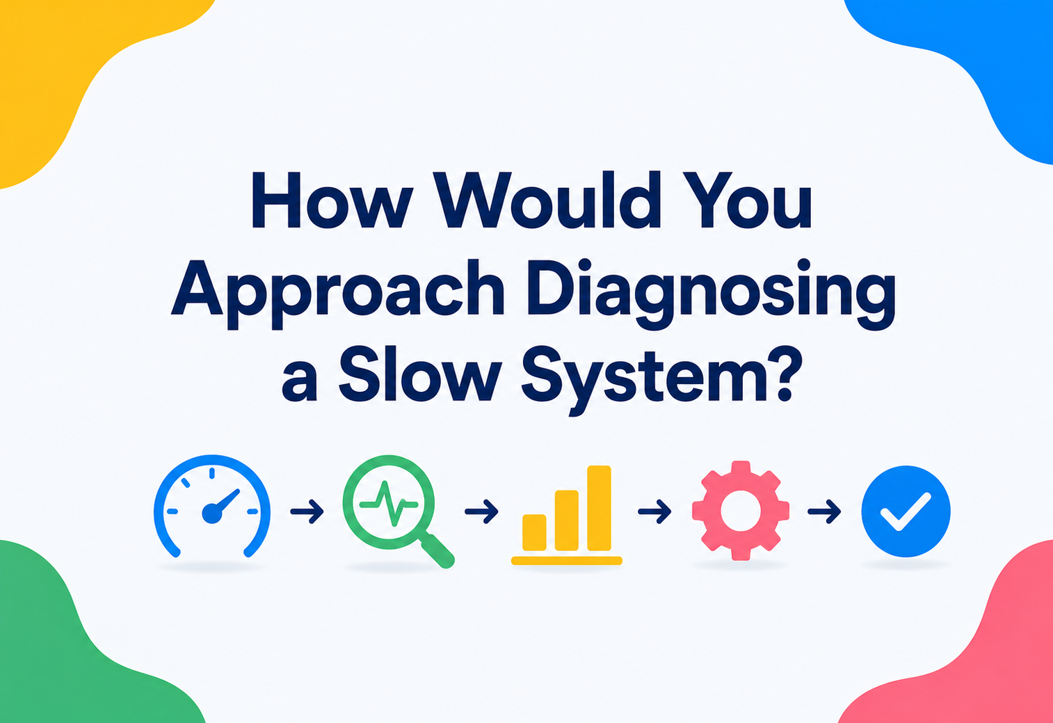
How Would You Approach Diagnosing a Slow System?
A complete, ground-up guide to finding out why a system is slow — from first principles and mental models to the tools, patterns, and real production stories that separate a guess from a diagnosis. Nineteen chapters, one steady discipline: measure first, hypothesise second, fix only what the evidence points at.
Introduction & History
Diagnosing a slow system is one of the oldest problems in computing, even though the tools have changed beyond recognition. It rewards the same instincts today that it rewarded on a mainframe in 1975 — a stubborn refusal to guess — but the surface area of “the system” has exploded.
Imagine a water pipe running into your house. One day, the water trickles out instead of flowing. You do not know why — maybe the main valve is half-closed, maybe there is a clog somewhere in the pipe, maybe a hundred neighbours are all using water at the same time and there simply is not enough to go around. A “slow system” is the software version of that trickle. Something that used to feel instant now makes people wait, and your job is to figure out which part of the pipe is the problem.
Diagnosing slow systems is one of the oldest problems in computing, even if the tools have changed beyond recognition. In the 1960s and 70s, mainframe operators watched physical dials and punch-card job queues to see when a machine was “thrashing” — spending more time managing memory than doing real work. In the 1980s and 90s, as Unix matured, tools like top, vmstat, and iostat gave engineers a window into CPU, memory, and disk activity on a single machine. That was enough when a “system” meant one computer.
Then the internet happened. A “system” stopped being one machine and became dozens, then thousands, of machines talking to each other over a network, spread across data centres and continents. A slow request today might pass through a load balancer, three microservices, two caches, a message queue, and a database replica before a user ever sees a result. The person diagnosing the problem in 2026 needs the same core instincts as the mainframe operator in 1975 — but a much bigger toolbox.
Diagnosing a slow system means methodically figuring out where time is being lost and why, instead of guessing. It is detective work: you gather clues (metrics, logs, traces), form a hypothesis, and test it until you find the real culprit.
It is worth sitting with why this skill is treated as its own specialty rather than “just debugging.” Debugging usually answers the question “why did this produce the wrong output?” Diagnosing a slow system answers a different question: “why did this produce the right output too slowly?” The code is not broken in the traditional sense — it eventually gets the correct answer — but something in the path it took cost more time than it should have. That distinction matters because the tools you reach for are different. A debugger that steps through code line by line is fantastic for logic bugs and nearly useless for a database that is fine most of the time but occasionally stalls for four seconds under load. You need tools that observe behaviour over time and under real conditions, not tools that freeze a single execution and inspect it.
The history also explains why the field can feel fragmented, with dozens of overlapping tools and vocabularies. Each era solved the problems of its own architecture. Mainframe-era engineers cared about job scheduling and memory paging because that is what mainframes did. The client-server era of the 1990s introduced the idea of “the network” as a first-class suspect — a query might be instant on the database server but slow for a user because of a saturated corporate WAN link. The web era added HTTP, browsers, and eventually JavaScript as new places for time to disappear. The cloud and microservices era, from roughly 2010 onward, exploded the number of hops a single request takes, which is why distributed tracing (Section 14) had to be invented — the old single-machine tools simply could not see across a network boundary.
Today’s engineer inherits all of these layers simultaneously. A single “slow checkout” ticket might genuinely require thinking about mainframe-era concepts (is the database thrashing on memory?), client-server concepts (is the network saturated between two internal services?), and cloud-native concepts (did an autoscaling event just replace half the fleet with cold, unwarmed instances?) all at once. That layered inheritance is exactly why Section 4 walks through the modern architecture stack before touching a single tool — you cannot diagnose what you cannot first picture.

Think of a slow system the way you would think of a slow tap: the water is still coming out, so nothing is technically broken, but somewhere between the reservoir and your kitchen, a valve is half-closed, a pipe is corroded, or the neighbourhood is drawing more than the main line can carry. The plumber’s job is not to change every pipe. It is to find the one narrow spot — and the same is true here.
The Problem & Motivation
Why does this deserve its own discipline instead of just “check the logs”? Because slowness is almost never caused by the thing you first suspect, and guessing wrong is expensive. Every minute an engineer spends chasing the wrong lead is a minute a real user is stuck watching a spinner — or worse, giving up and leaving.
The business cost is well documented. Amazon has said that every 100 ms of added latency can cost it around 1% in sales. Google found that a delay of just a few hundred milliseconds in search results measurably reduced how much people searched. These are not abstract engineering metrics; they translate directly into lost revenue, lost trust, and — in systems like healthcare or emergency services — real-world harm.
Why Structured Diagnosis Wins
- Finds the real bottleneck instead of the “obvious” one
- Produces evidence you can show teammates
- Builds a reusable mental model for next time
- Prevents wasted fixes that do not move the needle
Why Guessing Fails
- Fixes the symptom, not the cause
- Wastes engineering time on dead ends
- Can introduce new bugs while “fixing” performance
- Erodes trust when the same issue keeps returning
Motivation aside, there is also a simple truth: slowness is a symptom, not a diagnosis. “The checkout page is slow” tells you almost nothing about whether the problem is in the browser, the network, the application server, the database, or a third-party payment API. The rest of this guide builds the muscle to go from “it is slow” to “here is exactly why, and here is the fix.”
There is also a psychological trap worth naming: the “obvious culprit” bias. When a system slows down, the first instinct is almost always to blame whatever changed most recently in your own mental model — the piece of code you personally wrote last week, or the component you already distrust from a past incident. Sometimes that instinct is right. Often it is not, and confirmation bias quietly steers the investigation toward evidence that fits the existing suspicion while explaining away evidence that does not. A structured process, followed the same way every time, is the antidote. It forces you to look at the whole system before locking onto a theory.
There is a useful analogy here to medicine. A doctor does not prescribe medication the moment a patient says “I feel unwell.” They take vital signs, ask about symptoms, sometimes run tests, and only then form a diagnosis — and even then, they often treat the diagnosis as provisional, ready to revise it if the patient does not improve. Performance diagnosis works the same way: vital signs are your metrics, symptoms are what users report, tests are traces and profiles, and the “diagnosis” is a hypothesis you should be willing to abandon the moment better evidence contradicts it.
“It got fast again on its own” is not a diagnosis either — it is the system telling you that whatever caused the slowness is still lurking, ready to fire the next time the same conditions line up. A slowness you did not explain will come back on its own schedule.
Core Concepts
Before touching any tool, you need a shared vocabulary. These few terms show up constantly in performance work, and mixing them up leads directly to wrong conclusions.
It is worth building this vocabulary the way a mechanic builds vocabulary before touching an engine — not because the words themselves matter for their own sake, but because sloppy language leads directly to sloppy diagnosis. Someone who says “the server is slow” when they mean “the p99 latency for one specific endpoint is high” will chase the wrong lead almost every time, because “the server” implies every request everywhere is affected, while “one endpoint’s p99” points at something much narrower and easier to isolate.
These six terms are not independent trivia; they are deeply connected, and understanding how they relate to each other is more valuable than memorising any single definition. Latency and throughput trade off against each other under load — a system can often handle more throughput by accepting slightly higher latency per request (batching, queueing), or achieve lower latency per request by sacrificing some throughput (dedicating more resources to fewer concurrent requests). Utilisation and saturation are related but distinct: a resource can be highly utilised without being saturated (fully busy but keeping up with demand), or it can become saturated even at moderate utilisation if the arrival pattern is bursty rather than smooth. Errors interact with all of the above in a sneaky way — a system under enough stress will often start failing requests outright rather than completing them slowly, which can make raw latency numbers look artificially healthy even as the user experience gets dramatically worse.
Latency
How long a single request takes, start to finish. Measured in milliseconds. A page that takes 800 ms to load has 800 ms of latency.
Throughput
How many requests a system handles per unit of time — e.g., 500 requests per second. High throughput and low latency are both good, but they are different things.
Utilisation
How “busy” a resource is, e.g., CPU at 80% utilisation. High utilisation is not automatically bad — it can mean you are getting your money’s worth.
Saturation
Work queued up because a resource cannot keep up — e.g., processes waiting for CPU time. Saturation is the real warning sign, more than raw utilisation.
Errors
Requests that fail outright. A “slow” system that is secretly dropping requests may look fast because failed requests get counted as instant.
Percentiles (p50/p95/p99)
Averages hide pain. p99 latency tells you how slow the request was for the unluckiest 1% of users — often where the real story lives.
Two frameworks tie these together and are worth memorising:
- The USE Method (Brendan Gregg): for every resource, check Utilisation, Saturation, and Errors. It is built for hardware resources — CPU, memory, disk, network.
- The RED Method: for every service, track Rate (requests/sec), Errors (failed requests), and Duration (latency). It is built for services rather than hardware.
Do not confuse a high average latency with a widespread problem. A single slow database query hit by 1% of traffic can drag your average up while 99% of users are perfectly fine. Always look at the distribution, not just the mean.
Why Percentiles Beat Averages
Imagine 100 requests. Ninety-nine of them complete in 50 milliseconds. One takes 10 seconds because it happened to collide with a slow disk write. The average latency across those 100 requests is roughly 150 ms — which sounds mildly concerning but not alarming. Yet if that unlucky pattern repeats for every user roughly 1% of the time, then across a million requests a day, ten thousand real people are having a genuinely bad experience, and the average completely hides it. This is why performance teams talk in percentiles: p50 (median) tells you about the typical user, p95 tells you about a fairly unlucky user, and p99 (or even p99.9 at large scale) tells you about the truly unlucky ones — often the users who are also the most valuable, since power users and high-volume customers generate more requests and are statistically more likely to land in that unlucky tail.
A Gentle Introduction to Queueing
Most slowness, once you dig deep enough, is really a story about queues. A CPU core, a database connection pool, a thread pool, a network link — each is a resource that can only do one (or a few) things at a time, and anything that arrives while the resource is busy has to wait in line. Queueing theory shows something unintuitive: as utilisation approaches 100%, wait times do not increase gradually — they increase explosively. A resource at 70% utilisation might have barely any queueing delay, while the same resource at 95% utilisation can have wait times many times longer, even though utilisation only went up by 25 percentage points. This is why “the CPU is only at 90%, that is fine” can be a dangerously wrong read of a system that is actually one small traffic bump away from falling off a cliff.
Below 60–70% utilisation, queueing delay is usually negligible. Between 70% and 85%, it starts to notice. Above 90%, it starts to hurt. Above 95%, it can dominate everything else — and above 98%, a resource is effectively saturated even if the graph still says the number went up smoothly.
Architecture: Where Slowness Hides
A single user request today typically crosses many boundaries, and each one is a place time can be lost. Think of it as layers, like a cake — slowness can live in any layer, or in the seams between them.
Client / Browser
Slow JavaScript, unoptimised images, or render-blocking scripts on the user’s own device.
Network
DNS lookups, TLS handshakes, packet loss, or simply physical distance between user and server.
Load Balancer / Gateway
Misconfigured routing, connection pool exhaustion, or unhealthy backend targets.
Application Layer
Inefficient code, blocking I/O, thread pool starvation, garbage collection pauses.
External Dependencies
Third-party APIs, payment gateways, or partner services outside your control.
A skilled diagnostician does not start troubleshooting inside the application server just because that is the code they know best. They start at the edges and work inward — or, more efficiently, they use evidence (traces, metrics) to jump straight to the guilty layer.
A Worked Example: “The Dashboard Is Slow”
Say a user reports that an internal analytics dashboard takes eight seconds to load, when it used to take one. Walking the layers from Section 4 gives a checklist rather than a guess:
- Client: Did the frontend bundle grow larger in the last release? Is the browser rendering a huge, unpaginated table?
- Network: Is the user on a slow connection, or did a CDN edge node start missing cache and forwarding every request back to the origin?
- Load Balancer: Are health checks failing for some backend instances, funneling all traffic onto a shrinking pool of healthy ones?
- Application: Did a recent deploy introduce a loop that calls an internal API once per row instead of once per page?
- Data Layer: Did the underlying dataset simply grow, turning a once-fast query into a full table scan?
Notice that every one of these is plausible, and none of them can be ruled out by guessing. Only evidence — a trace showing which hop took eight of the eight seconds, or a query plan showing a table scan — can tell you which branch of that checklist is real. That is the whole point of the lifecycle in Section 6.
How Diagnostic Tools Work Internally
It helps to understand what is actually happening under the hood of the tools you will use, because it explains their trade-offs — and why a tool that is perfect for one situation is close to useless in another.
Sampling Profilers
A sampling profiler interrupts the running program at fixed intervals — say, every 10 milliseconds — and records exactly which line of code is executing at that instant. Do this thousands of times, and you get a statistical picture of where the program spends its time, similar to a pollster calling a sample of voters instead of everyone. It is low overhead (usually 1–3% slowdown) which makes it safe to run in production.
Instrumentation / Tracing
Instrumentation inserts explicit markers into the code — “this function started at time X” and “this function ended at time Y” — giving exact, complete data rather than a statistical estimate. It is more precise but adds more overhead, and someone has to add the instrumentation (or use an auto-instrumentation agent).
A Minimal Java Timing Example
Here is the simplest possible instrumentation — wrapping a suspect method with timers to get a first data point before reaching for heavier tools:
public class OrderService {

    public Order processOrder(Long orderId) {
        long start = System.nanoTime();

        Order order = loadOrder(orderId);            // suspect #1: DB call
        validateInventory(order);                    // suspect #2: downstream API
        Payment payment = chargeCustomer(order);     // suspect #3: external service

        long elapsedMs = (System.nanoTime() - start) / 1_000_000;
        if (elapsedMs > 500) {
            log.warn("Slow order {} took {}ms", orderId, elapsedMs);
        }
        return order;
    }
}This is intentionally crude — real systems use distributed tracing (covered in Section 14) — but the underlying idea is identical: measure boundaries, then narrow in on whichever boundary is slow.
A Special Case: Garbage Collection Pauses
Languages that manage memory automatically — Java, C#, Go, Python, and others — periodically run a garbage collector to reclaim memory that is no longer in use. Most of the time this is invisible. But under memory pressure, a garbage collector can trigger a “stop-the-world” pause, where every application thread freezes for anywhere from milliseconds to, in bad cases, several seconds, while the collector works. From the outside, this looks exactly like a random, unexplained latency spike — the code is not doing anything wrong, the database is not slow, the network is fine, but requests in flight during that window simply stall. Recognising the signature — a spike in latency that correlates with a sawtooth pattern in memory usage, confirmed by GC logs — is a specific, learnable skill, and it is a good example of why “read the metrics for this exact resource” beats “guess based on what usually causes slowness.”
// Enabling basic GC logging on the JVM (illustrative flags)
// -Xlog:gc*:file=gc.log:time,uptime:filecount=5,filesize=10M

// A pause line in the resulting log looks roughly like:
// [12.345s][info][gc] GC(42) Pause Young (Normal) 512M->128M(1024M) 45.231ms
Sampling profilers are the right tool when you can already reproduce the slowness and want to know where in the code time is being spent. Distributed tracing is the right tool when you do not yet know which service is slow. Reach for both eventually — but reach for the trace first when the request crosses network boundaries.
The Diagnostic Lifecycle
Diagnosing a slow system follows a repeatable lifecycle, whether you are debugging a laptop app or a global platform. Skipping steps is the single most common reason engineers chase the wrong fix.
Confirm and Quantify
Is it actually slow, for whom, how often, and compared to what baseline? Get numbers before touching anything.
Reproduce
Can you trigger the slowness on demand? A reproducible problem is a solvable problem.
Narrow the Layer
Use the architecture map from Section 4 to figure out which layer — client, network, app, data — is responsible.
Form a Hypothesis
State a specific, testable guess: “I believe the checkout API is slow because of database lock contention on the orders table.”
Test the Hypothesis
Use the right tool (profiler, trace, query plan) to prove or disprove it — do not stop at the first plausible-looking metric.
Fix and Verify
Apply the fix, then re-measure using the same method from step 1 to confirm it actually worked.
Prevent Recurrence
Add monitoring, alerts, or tests so the same issue is caught automatically next time.
Steps 4 and 5 — forming and testing a hypothesis — deserve extra attention because they are where most investigations go wrong. A weak hypothesis is vague and untestable: “the server seems overloaded.” A strong hypothesis is specific and falsifiable: “the API’s p99 latency rose because the connection pool to the payments database is exhausted during peak hours, causing requests to queue for a free connection.” The second version tells you exactly what to check — connection pool metrics — and exactly what would prove it wrong — if the pool has plenty of free connections during the slow window, the hypothesis is dead and you move to the next one.
It is tempting to stop at the first hypothesis that “fits.” Discipline means asking, even after you find supporting evidence: is there another explanation that also fits this same evidence? A spike in database CPU could mean an inefficient new query — or it could mean a completely unrelated batch job started running at the same time and is coincidental, not causal. The fix for correlation-versus-causation confusion is simple but often skipped: change one variable, re-measure, and see if the symptom actually moves.
Before shipping any fix, write down — in one sentence — exactly which metric you expect it to move, in which direction, and by roughly how much. If you cannot answer that, you are not verifying a hypothesis, you are hoping.
Trade-offs of Different Diagnostic Approaches
No single tool tells the whole story. Experienced engineers move fluidly between them — dashboards to spot the anomaly, tracing to localise it, and profiling to pin the exact line of code.
| Approach | Best For | Trade-off |
|---|---|---|
| Dashboards / Metrics | Spotting that something is wrong, fast | Tells you “what,” rarely “why” |
| Logs | Understanding specific events and errors | Can be noisy; needs good structure to search |
| Distributed Tracing | Pinpointing which service in a chain is slow | Requires instrumentation everywhere; storage cost |
| Profiling | Finding exactly which code is slow | Usually needs a reproducible case; some overhead |
| Load Testing | Finding limits before they hit production | Synthetic traffic does not always match real usage |
No single tool tells the whole story. Experienced engineers move fluidly between these — dashboards to spot the anomaly, tracing to localise it, and profiling to pin the exact line of code.
It helps to think of these tools as a funnel rather than a menu you pick one item from. Dashboards operate at the widest end of the funnel — cheap to check, covering the entire system at a glance, but only capable of telling you that something is wrong, rarely why. Logs and traces narrow the funnel, pointing at a specific service, a specific time window, or a specific request path. Profiling sits at the narrowest end — expensive to run broadly, but capable of pinpointing an exact function or even an exact line of code once you already know roughly where to look. Reaching for a profiler before checking a dashboard is like performing exploratory surgery before taking a patient’s temperature: technically thorough, but wildly inefficient, and it is a mistake even experienced engineers make when they are in a hurry and skip straight to the tool they are most comfortable with.
Dashboards → logs → traces → profiles. Move down the funnel only as fast as evidence pulls you. Every step you skip is a step you may end up walking back.
Performance & Scalability
Sometimes a system is not “buggy slow” — it is just doing more work than it was built for. Understanding scalability limits is core to diagnosis, because the fix for a bottleneck is different from the fix for genuine overload.
Amdahl’s Law
Amdahl’s Law says that the speedup from adding more parallel workers is capped by the portion of the work that cannot be parallelised. If 10% of a task must run sequentially, you can never get more than a 10x speedup no matter how many CPUs you throw at it. This is why “just add more servers” does not always fix slowness — if the bottleneck is a single-threaded lock, more servers change nothing.
Vertical vs. Horizontal Scaling
Vertical Scaling (bigger machine)
- Simple, no code changes
- Good for quick relief under load
- Works well for single-threaded bottlenecks
- Has a hard ceiling — one machine only gets so big
Horizontal Scaling (more machines)
- Scales almost indefinitely, if the workload is parallelisable
- Requires the app to be stateless or coordinated
- Adds network and consistency complexity
- Does nothing for single-threaded or single-writer bottlenecks
Adding servers to a system bottlenecked on a single database write-lock does not help — it just means more servers waiting in the same line. Confirm the bottleneck is actually parallelisable before scaling out.
Little’s Law: A Practical Capacity Formula
Little’s Law is a deceptively simple equation that connects three things you can usually measure: the average number of requests in a system (L), the average arrival rate of new requests (λ), and the average time each request spends in the system (W). The relationship is L = λ × W. In plain English: the number of requests being handled at any moment equals how fast they are arriving multiplied by how long each one takes. This becomes a genuinely practical diagnostic tool. If you know your target latency and your expected traffic rate, you can calculate exactly how much concurrent capacity — how many threads, how many database connections, how many worker processes — you actually need, instead of picking a pool size out of thin air and hoping.
If your service handles 200 requests per second (λ) and each request takes 250 ms on average (W), then at any moment you have on average 200 × 0.25 = 50 requests actively in flight. That is the minimum concurrent capacity you must design for — connection pools, worker threads, downstream client pools — before queueing delay starts to appear.
Identifying the True Bottleneck
A system is a chain of components, and a chain is only as fast as its slowest, most saturated link. The Theory of Constraints, borrowed from manufacturing, applies directly here: improving any part of the system that is not the current bottleneck produces no measurable improvement at all. Doubling the speed of your application servers does nothing if the real constraint is a single-threaded database write path. This is why the diagnostic lifecycle insists on evidence before action — optimising the wrong component is not a neutral mistake, it is wasted engineering time that could have gone toward the real fix.
High Availability & Reliability
Slowness and downtime are close cousins. A request that takes 30 seconds to fail is often worse than one that fails instantly, because it ties up connections, threads, and resources the whole time — a phenomenon sometimes called a “slow death” or “gray failure.” These are notoriously hard to detect because standard health checks often still report the system as “up.”
This is why timeouts, circuit breakers, and bulkheads (Section 15) matter as much for reliability as for pure speed — a slow dependency left unchecked can take down an otherwise healthy system.
Why “Gray Failures” Are So Hard to Catch
A traditional health check usually asks a simple yes-or-no question: can this service respond to a ping at all? A service experiencing a gray failure can answer that ping instantly while simultaneously failing or stalling on the actual work it is supposed to do — for example, a web server that responds to /health in one millisecond while every real request queues behind an exhausted database connection pool. Because the health check passes, orchestration systems keep sending it traffic, and load balancers keep it in rotation, even as users experience timeouts. Catching this requires health checks that exercise a realistic path through the system — touching the database, the cache, and any critical dependency — rather than simply confirming the process is alive.
The Cascading Failure Pattern
A single slow dependency rarely stays contained. If Service A calls Service B, and B slows down, requests to A start piling up waiting for B to respond. If A has a fixed thread pool, it eventually exhausts that pool entirely, meaning A becomes unresponsive to everyone — including callers who have nothing to do with B. That unresponsiveness then propagates to whatever calls A, and so on up the chain. A localised slowdown in one component can, within seconds, become a system-wide outage. Recognising this pattern during an incident — noticing that failures are spreading outward from a single origin point rather than appearing everywhere at once — often points investigators straight to the root cause.
A cascading failure is a traffic jam that started with a single stalled car in the far-left lane. Ten seconds after the stall, the left lane is stopped. A minute later, all three lanes are stopped, because drivers are merging. Two minutes later, cars a kilometre back have no idea a single stalled Honda is why they are late for dinner — and neither, at first, do you.
Security-Related Slowness
Not every slowdown is an innocent bug. Security issues frequently masquerade as performance problems, so a good diagnostician always keeps this possibility on the list.
Denial of Service (DoS/DDoS)
A flood of traffic — malicious or not — can saturate a system exactly like a legitimate traffic spike, just with intent behind it.
Algorithmic Complexity Attacks
Attackers craft inputs (e.g., pathological regex, hash collisions) designed to trigger worst-case, extremely slow code paths.
Credential Stuffing
Massive volumes of login attempts can quietly overload authentication services, showing up as “the login page is slow.”
Cryptomining Malware
Compromised servers running hidden mining processes show up first as unexplained, sustained high CPU usage.
The practical takeaway: if a slowdown does not match any deploy, traffic pattern, or known bug, checking access logs and traffic origin should be part of your standard checklist, not an afterthought.

Telling Legitimate Load Apart From an Attack
A sudden traffic spike from a viral social media post and a sudden traffic spike from a botnet can look nearly identical on a basic requests-per-second graph. The distinguishing signals usually live one level deeper: legitimate spikes tend to show a diverse mix of user agents, referrers, and geographic origins that roughly matches your normal audience, while attack traffic often clusters — many requests from a narrow IP range, an unusual user-agent string, or requests hitting only a single expensive endpoint rather than browsing naturally across the site. Building this kind of traffic fingerprinting into your monitoring, ahead of time, turns “is this an attack?” from a frantic guess during an incident into a quick lookup.
TLS and Encryption Overhead
It is also worth remembering that security infrastructure itself has a performance cost, and misconfigurations there are a frequent, non-malicious cause of slowness. A TLS handshake that should take one round trip can balloon to several if certificate chains are too long, if OCSP (certificate revocation) checks are slow, or if session resumption is not configured — adding real, measurable latency to every single new connection before a single byte of actual application data moves.
A slowdown that only appears on the very first request from a new client — and disappears on subsequent requests — is almost always a handshake, DNS, or connection-setup problem, not an application one. It is a signature worth learning to recognise on sight.
Monitoring, Logging & Metrics
This is the instrument panel that makes everything above possible. Without good observability, diagnosis is archaeology instead of investigation.
The Three Pillars of Observability
- Metrics: numeric time-series data (CPU%, request rate, latency) — cheap to store, great for dashboards and alerting.
- Logs: discrete, timestamped events — great for understanding exactly what happened at a specific moment.
- Traces: the end-to-end path of a single request across every service it touches — great for distributed systems (Section 14).
Set alerts on symptoms users feel (latency, error rate) rather than internal causes (CPU%). A server can run at 95% CPU and be perfectly healthy — what matters is whether requests are still fast and succeeding.
Structured Logging Matters More Than It Sounds
A log line like "order failed" is nearly useless when you are trying to correlate a slowdown across thousands of requests per second. Structured logs — emitted as key-value pairs or JSON, with a consistent trace ID attached — let you filter, aggregate, and join with metrics and traces automatically. The difference between free-text logs and structured logs is the difference between reading a diary by hand and being able to run a query against it.
{
  "timestamp": "2026-07-22T14:32:07Z",
  "level": "WARN",
  "service": "order-service",
  "trace_id": "8f3a1c9e-22b1",
  "message": "downstream call slow",
  "downstream": "inventory-service",
  "duration_ms": 4211,
  "order_id": "ORD-58231"
}trace_id links this event back to the exact request across every other service it touched.With logs shaped like this, answering “how many requests were slow because of the inventory service in the last hour, and were they all from the same customer segment?” becomes a query instead of a manual search through scrollback.
Golden Signals Dashboard
Google’s Site Reliability Engineering practice popularised four “golden signals” worth putting on every service’s primary dashboard: latency, traffic, errors, and saturation. Together they answer the two most urgent questions during an incident — is it broken, and is it slow — without requiring anyone to dig through raw logs just to get oriented.
Cloud & Deployment Considerations
Cloud environments introduce their own special flavours of slowness that do not exist on a machine sitting under your desk.
Noisy Neighbours
On shared virtual hardware, another tenant’s heavy workload can silently steal CPU or I/O from yours.
Cold Starts
Serverless functions and auto-scaled containers can take real time to initialise before serving their first request.
Autoscaling Lag
New capacity takes minutes to spin up — a traffic spike can overwhelm a system before it finishes scaling.
Cross-Region Latency
A service call that quietly crosses a regional boundary adds tens or hundreds of milliseconds of pure network distance.
When diagnosing a cloud-hosted system, always ask: did anything about the underlying infrastructure change — a deploy, an instance type, an autoscaling event, a region failover — around the time the slowness began?
Container Resource Limits
In containerised environments, a container can be silently throttled by its own CPU or memory limits well before the underlying host machine looks busy at all. From inside the container, this shows up as strangely inconsistent latency with no obvious cause; from the orchestration layer’s point of view, it is working exactly as configured. Checking a container’s own throttling metrics — not just the host machine’s overall CPU graph — is a step that is easy to skip and often exactly where the answer is hiding.
Managed Service Quotas and Throttling
Cloud providers frequently impose rate limits or quotas on managed services — API request limits, database IOPS caps, network bandwidth ceilings — that exist specifically to protect shared infrastructure. When a system approaches one of these limits, requests are not rejected outright; they are often just delayed or queued, which looks identical to organic slowness from the application’s point of view. Cloud provider dashboards for “throttled requests” or “throughput exceeded” events are an easy, high-value check that is frequently overlooked because the slowdown does not originate in your own code at all.
Cross-availability-zone traffic is often invisible in application-level metrics but is real, measurable latency on every hop. A microservice that used to run beside its database in one zone, and now runs in a different zone after a failover or a routine rebalance, can look mysteriously slower without a single code change.
Databases, Caching & Load Balancing
In practice, an enormous share of “slow system” tickets trace back to these three components. They deserve special attention.
Databases
- Missing indexes: the database scans an entire table instead of jumping straight to the relevant rows.
- Lock contention: multiple transactions fight over the same rows, forcing others to wait.
- Replication lag: a read replica returns stale or delayed data because it has not caught up with the primary.
- N+1 queries: code that issues one query per item in a loop instead of a single batched query.
Caching
Caching helps enormously — until it does not. A “cache stampede” happens when a popular cached item expires and thousands of requests hit the database simultaneously trying to refill it, momentarily turning a fast system into a very slow one.

Load Balancing
An unevenly balanced load — where one server gets far more traffic than its peers due to a bad hashing strategy or a “sticky session” — can make part of your fleet look overloaded while the rest sits idle.
Adding a cache to “fix” a slow database query treats the symptom. If the underlying query is fundamentally inefficient, you have just delayed the pain until the cache misses or expires.
Reading a Query Plan, in Plain Terms
Every relational database can explain how it intends to execute a query before running it — usually via an EXPLAIN command. The output looks intimidating, but the core question is always the same: is the database using an index to jump straight to the rows it needs, or is it scanning every row in the table one by one? The difference in cost is enormous. Looking something up in an indexed table of ten million rows might touch a few dozen rows internally; scanning the same table touches all ten million. As a table grows, a missing index does not degrade performance gently — it can turn a 10-millisecond query into a 10-second query almost overnight, once the table crosses a size where the scan becomes noticeable.
-- Before: no index on customer_email, full table scan
EXPLAIN SELECT * FROM orders WHERE customer_email = 'user@example.com';
-- Seq Scan on orders  (cost=0.00..184521.00 rows=1 width=120)

-- After: adding an index
CREATE INDEX idx_orders_customer_email ON orders(customer_email);

EXPLAIN SELECT * FROM orders WHERE customer_email = 'user@example.com';
-- Index Scan using idx_orders_customer_email  (cost=0.43..8.45 rows=1 width=120)
The cost estimates above (184,521 versus 8.45, in the database’s own internal units) illustrate exactly the kind of order-of-magnitude difference that separates “instant” from “the page hangs for ten seconds.”
APIs, Microservices & Distributed Tracing
Microservices multiply the number of places a single request can slow down. A checkout request might touch ten services; if any one of them is slow, the whole request is slow — and worse, that slowness can cascade.
Without distributed tracing, that 4,800 ms shows up as “checkout is slow” with no clue that Inventory Service is the actual culprit. A trace, using a shared request ID (trace ID) passed between every service, lets you see the whole waterfall and immediately spot the outlier.
A Simple Trace-Context Java Snippet
public class TraceContext {
    private static final ThreadLocal<String> TRACE_ID = new ThreadLocal<>();

    public static void start(String incomingTraceId) {
        TRACE_ID.set(incomingTraceId != null
            ? incomingTraceId
            : java.util.UUID.randomUUID().toString());
    }

    public static String get() {
        return TRACE_ID.get();
    }
}

// Every outbound call forwards the same trace ID:
httpClient.header("X-Trace-Id", TraceContext.get());This is the seed of what tools like Jaeger, Zipkin, and OpenTelemetry do at scale — automatically, across every service, with timing built in.
Why Traces Are Sampled, Not Kept Forever
At real scale — millions of requests per hour — recording a full detailed trace for every single request would be prohibitively expensive to store and slow to write. Most tracing systems therefore sample: they might record every trace in detail for the first minute after a deploy (when problems are most likely), then drop to recording only 1% of normal traffic, while always keeping 100% of traces that hit an error or exceed a latency threshold. This “tail-based sampling” strategy — deciding whether to keep a trace only after seeing how it turned out — means you rarely lose visibility into exactly the requests you would want to investigate, while keeping storage costs manageable for the overwhelming majority of boring, fast, successful requests.
The N+1 Problem in a Microservices World
The classic N+1 query problem (Section 13) has a distributed cousin. A service handling a request for “show me this user’s orders with product details” might naively call the Order Service once, then call the Product Service once per order returned — turning what should be two network calls into twenty-one for a user with twenty orders. Each of those calls carries its own network round-trip latency, and they add up fast, especially if the calls happen sequentially rather than in parallel. A trace waterfall view makes this pattern immediately visible: a long, repetitive staircase of near-identical calls to the same downstream service is close to a textbook signature for this exact anti-pattern, and the fix is almost always to batch the request into a single call that accepts a list of order IDs.
Design Patterns & Anti-patterns
A small set of patterns show up over and over in resilient, fast systems — and the same set of anti-patterns show up over and over in the incident post-mortems of systems that are neither.
Patterns That Help
- Circuit Breaker: stops calling a failing/slow dependency for a cooldown period
- Bulkhead: isolates resources so one slow component cannot starve everything else
- Timeout + Retry with Backoff: fails fast instead of hanging indefinitely
- Caching with TTL Jitter: avoids synchronised cache expiry (stampedes)
Anti-patterns That Hurt
- No Timeouts: one hung dependency freezes everything waiting on it
- Chatty Services: many small calls instead of one batched call
- Synchronous Everything: blocking calls stacked up with no async option
- Unbounded Queues: work piles up invisibly until memory runs out
A Minimal Circuit Breaker in Java
The idea behind a circuit breaker is borrowed directly from household electrical circuit breakers: when something downstream is failing or too slow too often, stop sending it traffic for a while so it has room to recover, and so your own system does not get dragged down waiting on it.
public class SimpleCircuitBreaker {
    private int failureCount = 0;
    private final int threshold = 5;
    private long openedAt = 0;
    private final long cooldownMs = 30_000;
    private boolean open = false;

    public boolean allowRequest() {
        if (open && System.currentTimeMillis() - openedAt > cooldownMs) {
            open = false;          // try again after cooldown ("half-open")
            failureCount = 0;
        }
        return !open;
    }

    public void recordFailure() {
        failureCount++;
        if (failureCount >= threshold) {
            open = true;
            openedAt = System.currentTimeMillis();
        }
    }

    public void recordSuccess() {
        failureCount = 0;
    }
}threshold failures accumulate, calls fail fast for cooldownMs before a cautious retry — buying the downstream service room to recover.Once the breaker trips open, calls fail fast — instantly, instead of hanging for a full timeout — which protects the caller’s own thread pool and gives the downstream service breathing room to recover before traffic resumes.
Instead of setting every cache entry to expire in exactly 60 seconds, expire in a random value between 55 and 65 seconds. That small change alone prevents the synchronised stampede where thousands of expiring entries all miss at the same instant.
Best Practices & Common Mistakes
A short set of habits that, held consistently, prevent more incidents than any single clever fix ever will — and the mirror-image set of mistakes that keep showing up in post-mortems.
Best Practices
- Always measure before and after a fix — “it feels faster” is not evidence.
- Look at percentiles (p95/p99), not just averages.
- Check what changed recently: deploys, config, traffic patterns, infrastructure.
- Keep a runbook of past incidents — most “new” slowdowns are repeats.
Common Mistakes
- Jumping straight to code changes before confirming where the time is actually going.
- Trusting a single dashboard without cross-checking traces or logs.
- Testing fixes only in staging, where traffic and data volume do not match production.
- Ignoring the client side and assuming the server is always the bottleneck.
A Quick Pre-Investigation Checklist
Before diving into tools, five quick questions often narrow the search space dramatically, and cost almost nothing to ask:

What changed?
Deploys, config, feature flags, infrastructure, or third-party dependency versions around the time it started.
Who is affected?
Everyone, one region, one customer segment, or one specific feature — the pattern itself is a clue.
When did it start?
A sharp step-change points to a specific event; a gradual drift points to organic growth or a slow leak.
Is it truly slow, or truly failing?
Confirm whether requests are completing late or timing out and silently retried, which can masquerade as slowness.
Has this happened before?
Check past incident records — many “new” problems are recurring ones with a known fix already documented.
Nine out of ten sudden slowdowns correlate in time with something the team itself deployed, configured, or turned on — even when the connection is not obvious. Checking the last two hours of change history is often the fastest way to a working hypothesis.
Real-World Case Studies
The following patterns are drawn from public engineering writing by teams at scale — not because these are the only companies who diagnose slowness well, but because they have documented their playbooks openly enough that everyone else can learn from them.
Netflix
Popularised chaos engineering partly to surface hidden slow-dependency cascades before they hit real users, deliberately injecting latency into services to test resilience.
Amazon
Publicly tied page-load latency directly to revenue, driving an obsession with p99 latency across every team, not just averages.
Pioneered the USE and “four golden signals” (latency, traffic, errors, saturation) approach to monitoring at massive scale via its Site Reliability Engineering practice.
Uber
Built extensive distributed tracing infrastructure (Jaeger, which it open-sourced) specifically because a single ride request touches dozens of microservices.
Etsy
Known for a strong culture of blameless post-mortems focused on “why did our monitoring not catch this sooner,” improving diagnosis speed over time.
A Closer Look: The Cascading Timeout Story
A pattern that has repeated, in some form, at nearly every large tech company at least once: a downstream service — say, a recommendation engine — starts responding slowly due to an unrelated database issue. The service calling it has no timeout configured, or an extremely generous one, so requests to the front-end service start piling up waiting on responses that never come quickly. Within minutes, the front-end service’s own thread pool is exhausted by requests stuck waiting, and it stops responding to anything at all — including requests that have nothing to do with recommendations, like the login page or the homepage. What began as a narrow, contained slowdown in one non-critical feature becomes a full site outage. The post-mortem lesson is almost always the same: every external call needs an explicit, sane timeout, and every service needs isolation (a bulkhead, from Section 15) so that one dependency’s bad day cannot sink the whole ship.
A Closer Look: The Silent Index Regression
Another recurring story: a database table grows steadily for months with no incident, until one day a query that always ran in milliseconds suddenly takes seconds. Nothing in the application code changed. The real cause is usually that the query optimiser’s statistics or execution plan flipped once the table crossed some threshold — deciding, for instance, that a full table scan had become cheaper than using an existing index because the table’s shape had changed enough. These regressions are notoriously hard to catch with code review alone because the code never changed; only the data did. Regularly reviewing slow-query logs, rather than waiting for a user complaint, is usually how these get caught before they become an incident rather than after.
Both stories share the same root pattern: a small, contained problem in one place, allowed to grow because nothing in the design forced it to stay contained. Timeouts, bulkheads, and slow-query alerts are not glamorous engineering. They are the seatbelts that keep a small stall from becoming a system-wide crash.
Frequently Asked Questions
Short, direct answers to the questions engineers ask most often when they start taking performance diagnosis seriously as a discipline of its own.
Is high CPU usage always a problem?
No. High utilisation can mean the system is efficiently using the resources it paid for. The warning sign is saturation — work queueing up because there is not enough CPU to go around — not utilisation alone.
Should I always start diagnosis at the database?
No, though it is a common starting guess because it is often the culprit. Start with evidence — a trace or metric that points to a layer — rather than habit.
How do I diagnose an intermittent slowdown that I cannot reproduce?
Lean on always-on observability (logs, traces, metrics) rather than live debugging. Look for correlation with time of day, deploys, or specific request types across historical data.
What is the very first thing to check?
Whether anything changed recently — a deploy, a config change, a traffic spike, an infrastructure event. Most sudden slowdowns correlate with a specific change.
How is diagnosing a slow system different from load testing?
Load testing is proactive — you generate synthetic traffic to find limits before real users do. Diagnosis is usually reactive — something is already slow, and you are working backward from a real symptom. The two feed each other: a diagnosis often reveals a limit worth load-testing for next time, and a load test often surfaces a bottleneck worth diagnosing before it ships.
Do I need distributed tracing for a small system?
Not necessarily. If your entire system is one application talking to one database, a profiler and good logging often go a long way, and tracing infrastructure can be more operational overhead than it is worth. Tracing earns its cost once a request routinely crosses more than two or three network hops.
How do I know when to stop digging and just ship a fix?
When your hypothesis has been tested against real evidence and the fix’s expected impact is well understood — not when you have simply run out of patience. Shipping an untested guess under time pressure often trades a known slow system for an unknown one.
What is the smallest habit that improves diagnosis the most?
Writing every incident’s root cause and fix into a searchable runbook. Most “new” slowdowns turn out to be old slowdowns wearing different clothes, and a searchable runbook turns a two-hour investigation into a two-minute lookup.
Summary & Key Takeaways
Diagnosing a slow system is a discipline, not a guess. It rewards patience, evidence, and a mental map of every layer a request passes through.
What is worth remembering
- Slowness is a symptom — your job is to find the specific, provable cause behind it, not to react to the symptom itself.
- Follow the lifecycle: confirm, reproduce, narrow, hypothesise, test, fix, verify, prevent. Skipping steps is the single most common reason engineers chase the wrong fix.
- Use percentiles, not averages — the worst-case user often tells the real story, and the average frequently hides it.
- Combine metrics, logs, traces, and profiling — no single tool sees everything, and the funnel from broad to narrow is how experienced engineers move fast.
- Remember security, cloud infrastructure, and cascading dependencies as possible causes, not just “slow code” — the answer is often outside the code entirely.
- Every diagnosis should end with prevention — better monitoring, alerts, or safeguards for next time, so the same incident does not need diagnosing twice.
- Utilisation is not saturation, and 90% busy is very different from 95% busy — queueing delay grows explosively near the limit.
- Timeouts and bulkheads are not glamorous, but they are the seatbelts that keep one slow dependency from taking down the whole system.
The engineers who consistently diagnose slow systems well are almost always the ones who refuse to guess — who move from “it feels slow” to “here is the specific hop, the specific metric, and the specific fix,” one piece of evidence at a time, no matter how much time pressure the room is under.