What Is Queueing Theory? — Why It Is the Hidden Math Behind Every Scalable System
Every system that handles more than one request at a time is secretly a queueing system. Learn the math, the intuition, and the production patterns that keep Netflix, Amazon, and Uber running smoothly under load — from Erlang’s 1909 switchboard formulas to today’s Kubernetes autoscalers.
Introduction & History
Every backend engineer eventually meets the same uncomfortable moment: a system that looks perfectly healthy on the dashboard suddenly becomes unusable. The oldest, most respectable branch of mathematics that explains why has a name — queueing theory — and it has been quietly running in the background of civilisation since 1909.
Imagine you walk into a coffee shop. There is one person making coffee, and a line of customers waiting. Sometimes the line is short, sometimes it stretches out the door. What decides how long you wait? It is not magic. It is math — and that math has a name: queueing theory.
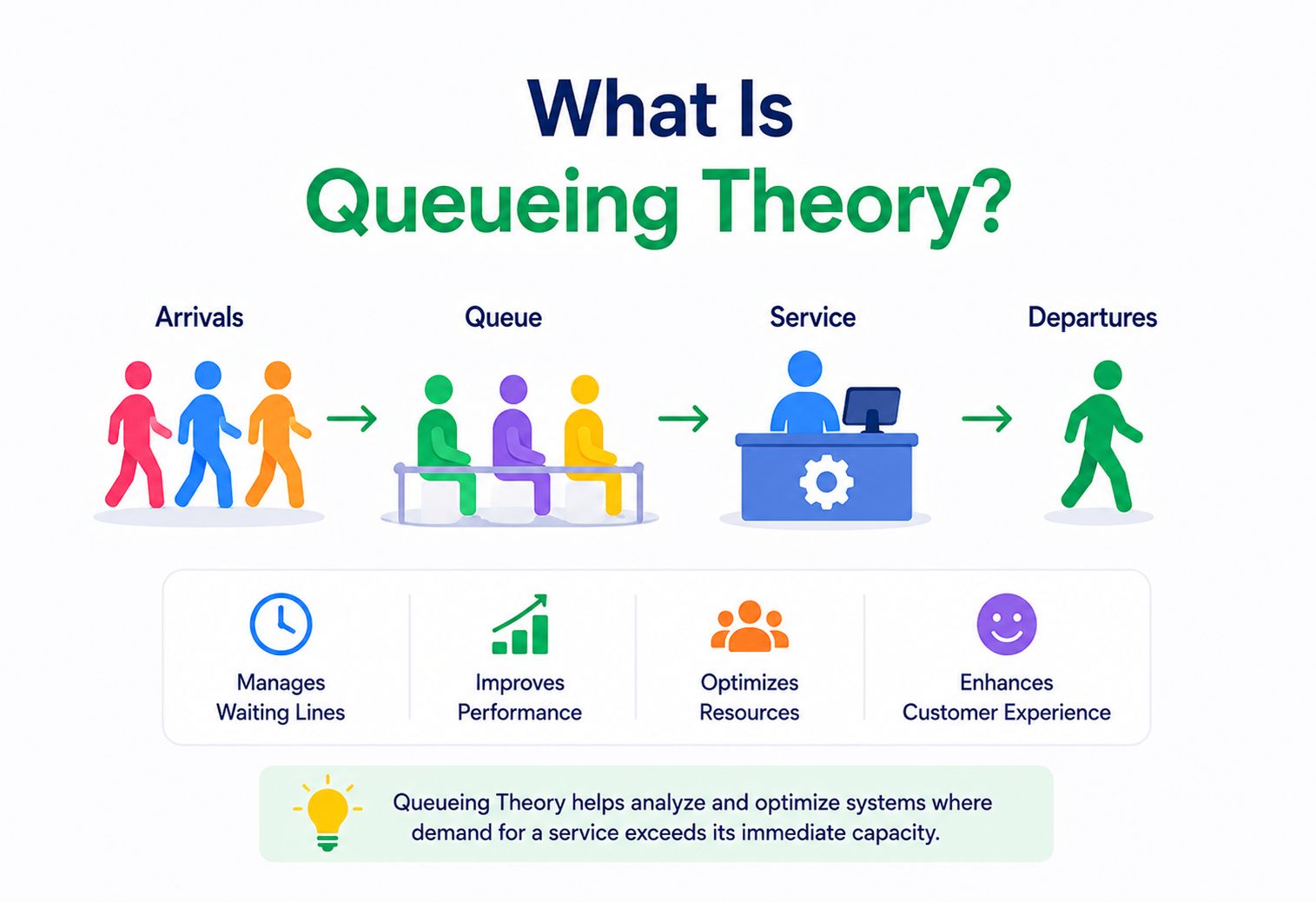
Queueing theory is the mathematical study of waiting lines (queues). It answers questions like: How long will something have to wait? How many things will be waiting at once? What happens if we add one more server (or barista, or CPU core, or database connection)? These are exactly the questions that keep backend engineers awake at night, because every computer system that serves more than one request at a time is, underneath the code, a queueing system.
The story of queueing theory does not start in a data centre. It starts in 1909, in Copenhagen, Denmark, with a Danish engineer named Agner Krarup Erlang, who worked for the Copenhagen Telephone Company. Back then, telephone calls were connected by human operators using physical switchboards. Erlang’s employer had a very practical problem: how many telephone lines and operators did they need so that customers did not wait too long — without buying far more equipment than necessary?
Erlang treated incoming calls as random arrivals and used probability theory to calculate the chance that a caller would have to wait, and for how long. His formulas were so accurate and so useful that they are still used today to size telephone trunks, call centres, and yes, modern software systems. In his honour, the unit used to measure telephone traffic is literally called the “Erlang.”
Over the next century, queueing theory grew from telephone networks into a general branch of applied probability and operations research. It found homes in traffic engineering (how many toll booths does a highway need?), hospital design (how many beds should an ER have?), manufacturing (how many machines on an assembly line?), and eventually, computer science. When computers started serving multiple users and multiple requests through shared resources — a CPU, a disk, a network link, a database connection pool — the exact same mathematics applied. A web server handling HTTP requests is, mathematically, no different from Erlang’s switchboard handling phone calls.
If you have ever wondered why a system that “should” handle the load starts timing out the moment traffic crosses some threshold — even though average load looks fine — queueing theory is the reason. It explains a counter-intuitive but critical truth: systems do not fail gracefully as they approach their limit; they fail exponentially. Understanding why is the difference between an engineer who reacts to outages and one who prevents them.
The Problem & Motivation — Why Do We Need This?
Let us start with a question every engineer eventually asks: “My server can process 100 requests per second on average, and I am only receiving 90 requests per second. Why is it falling over?”
This is one of the most common and most misunderstood problems in backend engineering. The intuitive (and wrong) answer is: “90 is less than 100, so we have 10% headroom, we should be fine.” The queueing-theory answer is: “You are dangerously close to collapse, and here is exactly why.”
2.1 The core problem: randomness
Requests do not arrive in a smooth, predictable, evenly-spaced stream. They arrive in bursts. Ten users might click “checkout” in the same second, then nothing for three seconds, then five more arrive. Similarly, the time it takes to process each request is not a fixed number — some requests are simple and fast, others hit a slow code path, a cold cache, or a garbage collection pause.
This double randomness — random arrival times and random service times — is the entire reason queues form at all. If every request arrived at a perfectly fixed interval and took a perfectly fixed amount of time to process, and that time was less than the interval, no queue would ever form. But real systems are never that clean, and queueing theory exists precisely to model this randomness mathematically, rather than guess about it.
The toll booth
Think of a single toll booth on a highway. On average, one car arrives every 6 seconds, and the booth takes 5 seconds to process a car. On average, this looks fine — the booth is idle for 1 second between cars. But cars do not arrive exactly every 6 seconds. Sometimes three cars arrive within 2 seconds of each other. Now a queue forms, and it takes time to dissolve, even though the “average” says everything should be fine.
The checkout API
A checkout API can process 100 requests / second on average. During a flash sale, requests do not arrive smoothly — they spike when a popular product goes live. Even if the average stays under 100 / sec, these bursts create temporary overload, and because queues built during a burst take time to drain, latency stays high even after the burst passes.
2.2 Why “average load” lies to you
Dashboards love to show average CPU usage, average requests per second, and average response time. But averages hide the shape of the traffic. A system running at 60% average CPU can still have moments where it is at 100% for several seconds — and during those moments, requests queue up, and if the queue is unbounded, memory grows and latency explodes.
This is precisely the gap that queueing theory fills: it does not just tell you the average behaviour, it tells you about variance, worst-case waiting time, and the probability of overload — the numbers that actually determine whether your users have a good experience or see spinning loaders and timeouts.
Netflix, Amazon, and Uber do not run their systems at “the average load their servers can handle.” They run them at a fraction of theoretical maximum capacity — often 50–70% — precisely because queueing theory shows that latency does not increase linearly as you approach 100% utilisation. It increases explosively. We will prove this with real math in the next sections.
Core Concepts — The Building Blocks
Before we can apply queueing theory to system design, we need a shared vocabulary. Every concept here is simple on its own — the power comes from how they combine.
3.1 Arrival Rate (λ, “lambda”)
The arrival rate is how many requests (or customers, cars, phone calls) arrive per unit of time, on average. We use the Greek letter lambda (λ) for it. If your API receives 200 requests per second on average, then λ = 200 / sec.
Coffee shop
λ is how many customers walk into the coffee shop per minute.
API traffic
λ is your API’s requests-per-second, as seen in your load balancer’s metrics.
3.2 Service Rate (μ, “mu”)
The service rate is how many requests a single server (one thread, one worker, one database connection) can complete per unit of time, on average, if it never sat idle. We use the Greek letter mu (μ). If one worker thread can finish a task in 10 milliseconds, its service rate is μ = 100 / sec (1000 ms / 10 ms).
3.3 Utilisation (ρ, “rho”)
Utilisation is the fraction of time a server is busy, and it is the single most important number in queueing theory. It is calculated as:
where c is the number of servers (workers). If λ = 80 requests / sec and one server can handle μ = 100 requests / sec, then with one server, ρ = 80 / 100 = 0.8, meaning the server is busy 80% of the time. Utilisation must always stay below 1 (100%) for a queue to remain stable — if ρ ≥ 1, the queue grows forever because work arrives faster than it can be finished.
As ρ approaches 1, average wait time does not increase gently — it increases toward infinity. This is the mathematical root of why systems “suddenly” become slow near peak load, and why capacity planning obsesses over keeping utilisation comfortably below 100%.
3.4 Little’s Law — the most important equation in system design
Little’s Law, proven by John Little in 1961, is beautifully simple and applies to almost any stable queueing system, regardless of arrival patterns or service time distributions:
Where L is the average number of items in the system (waiting + being served), λ is the average arrival rate, and W is the average time an item spends in the system.

The restaurant
If a restaurant seats 5 new customers per minute (λ = 5 / min), and each customer stays for 40 minutes on average (W = 40 min), then on average there are L = 5 × 40 = 200 customers in the restaurant at any given moment. This tells the owner exactly how many chairs are needed.
The API
If your API receives 500 requests / sec (λ = 500), and each request takes 200 ms = 0.2 sec on average to fully process (W = 0.2), then on average there are L = 500 × 0.2 = 100 requests “in flight” in your system at any moment. This tells you exactly how many concurrent connections, threads, or memory buffers you need to provision.
Little’s Law is used constantly in production capacity planning: given a target latency (W) and expected traffic (λ), you can calculate exactly how much concurrency (L) your system must support — and from there, how many servers, threads, or connections you need.
3.5 Kendall’s notation: the shorthand for describing queues
Queueing systems are classified using a compact notation invented by David Kendall in 1953, written as A/S/c (sometimes extended to A/S/c/K/N/D):
| Symbol | Meaning | Common Values |
|---|---|---|
| A | Arrival process (how arrivals are distributed) | M = Markovian / random (Poisson process) |
| S | Service time distribution | M = random (exponential), D = deterministic (fixed) |
| c | Number of servers | 1, 2, 3, … or ∞ |
| K | System capacity (max queue size, optional) | a number, or ∞ if unbounded |
The most famous and most useful model in system design is M/M/1: random arrivals, random (exponentially distributed) service times, and a single server. It is the simplest realistic model of a single-threaded service, a single database connection, or a single CPU core processing one task at a time. M/M/c extends this to c parallel servers — exactly like a thread pool or a fleet of application server instances behind a load balancer.
3.6 Queue length, wait time, and response time
It is important to separate three related but distinct numbers, because production dashboards often blur them together:
- Queue length (Lq): how many requests are waiting, not yet being served.
- Wait time (Wq): how long a request waits before service starts.
- Response time / sojourn time (W): total time in the system, i.e. wait time + actual service (processing) time.
When your monitoring shows “p99 latency spiked,” it is almost always because Wq spiked — the actual processing time per request (service time) usually stays constant; it is the waiting that balloons.
3.7 The Poisson process: why “random arrivals” has a precise meaning
When queueing theory says arrivals are “random,” it usually means they follow a Poisson process — a specific, well-studied mathematical pattern where events happen independently of one another, at a constant average rate, with no “memory” of when the last event occurred. This might sound abstract, but it matches real-world request traffic surprisingly well: whether or not a request arrives in the next millisecond has nothing to do with whether one arrived in the previous millisecond (unless there is a specific correlated cause, like a scheduled batch job or a retry storm).
Raindrops on pavement
Raindrops hitting a specific square foot of pavement during light, steady rain follow roughly a Poisson process — each drop’s arrival is independent of the others, and on average you can predict how many land per minute, but you cannot predict exactly when the next one falls.
Website traffic
Requests from thousands of independent users browsing a website, each making their own unrelated decisions about when to click, closely approximate a Poisson process at the aggregate level — which is exactly why Erlang’s century-old telephone math still applies to modern web traffic.
A useful property of Poisson-driven systems, called PASTA (Poisson Arrivals See Time Averages), is that a randomly arriving request, on average, experiences the system exactly as an outside observer taking a snapshot at a random moment would see it. This is why steady-state average metrics (like average queue length) are meaningful predictors of what an actual incoming request will experience — a property that does not hold for many non-Poisson arrival patterns, such as tightly scheduled batch jobs.
3.8 Probability of waiting: P(wait > 0)
Beyond averages, queueing theory can answer sharper questions like: “What is the probability that a request has to wait at all, rather than being served immediately?” For an M/M/1 system, the probability the server is idle (and thus a new arrival is served instantly) is simply 1 − ρ, and the probability an arriving request must wait is ρ itself. For M/M/c systems with multiple servers, this probability is given by the Erlang C formula — the same formula Erlang derived in 1909 to size telephone exchanges, and the same formula many call-centre staffing tools still use today to calculate how many agents are needed to keep expected wait times under a target threshold.
Architecture & Components — Where Queues Hide in Every System
Once you start looking for queues, you find them everywhere in a software system — often disguised under a different name. Recognising them is the first step to designing around them deliberately instead of accidentally.
| What it is called | What it actually is | Servers (c) |
|---|---|---|
| Thread pool | Requests queue for an available thread | Number of threads |
| Database connection pool | Queries queue for a free connection | Pool size |
| Load balancer backlog | Connections queue before being routed | Backend instance count |
| Message broker (Kafka, SQS, RabbitMQ) | An explicit, durable queue | Number of consumers |
| CPU run queue / OS scheduler | Processes / threads queue for CPU time | Number of CPU cores |
| Network switch buffer | Packets queue before transmission | Link bandwidth |
| TCP backlog (accept queue) | Incoming connections queue before accept() | Listener capacity |
A single user request in a modern distributed system typically passes through five or six of these queues in sequence — the load balancer, the TCP accept queue, the application thread pool, the database connection pool, and possibly a downstream message queue. Each one adds its own waiting time, and these waiting times add up.
4.1 Explicit vs. implicit queues
It helps to separate queues into two categories:
- Explicit queues are ones you deliberately design and can see: message brokers like Kafka, RabbitMQ, or Amazon SQS. You choose their capacity, their consumers, and their behaviour when full.
- Implicit queues are ones that exist whether you designed for them or not: thread pools, connection pools, CPU schedulers, network buffers. They are invisible until they overflow — and by then, you are already in an incident.
Good system design does not eliminate queues — that is impossible, since queues are how systems absorb randomness. Good system design makes queues explicit, bounded, observable, and intentional, rather than leaving them implicit, unbounded, and invisible until they cause an outage.
Internal Working — The Math That Explains “Sudden” Slowdowns
Now let us derive the formula that explains one of the most important and counter-intuitive truths in system design: why latency explodes as utilisation approaches 100%, instead of increasing smoothly.
5.1 The M/M/1 waiting time formula
For the simplest realistic model — a single server, random arrivals, random service times (M/M/1) — the average time a request spends waiting in the queue before being served is:
Look closely at the denominator: (1 − ρ). As ρ (utilisation) climbs toward 1 (100%), this term approaches zero, and since it is in the denominator, Wq shoots toward infinity. This single term is the mathematical explanation for why systems that look “almost fine” on a dashboard can become unusable within seconds when traffic ticks up just a little further.
| Utilisation (ρ) | Relative Wait Time | What It Feels Like |
|---|---|---|
| 50% | 1× baseline | Smooth, snappy |
| 70% | 2.3× | Noticeably slower under load |
| 80% | 4× | Users start complaining |
| 90% | 9× | Alerts firing, timeouts begin |
| 95% | 19× | Cascading failures likely |
| 99% | 99× | System effectively down |
This is exactly why experienced architects target 60–70% utilisation for capacity planning, not 95%. The “spare” 30% is not waste — it is what absorbs the natural randomness (burstiness) of real traffic without wait times spiralling.
5.2 Calculating it yourself: a Java Little’s-Law calculator
Here is a small, self-contained Java utility that implements Little’s Law and the M/M/1 waiting-time formula — useful for back-of-the-envelope capacity planning before you provision real infrastructure.
public class QueueingCalculator {

    /**
     * M/M/1 average wait time in queue (before service starts).
     * @param arrivalRate  lambda, requests per second
     * @param serviceRate  mu, requests per second a single server can handle
     * @return average wait time in seconds
     */
    public static double averageWaitTime(double arrivalRate, double serviceRate) {
        double rho = arrivalRate / serviceRate;
        if (rho >= 1.0) {
            throw new IllegalStateException(
                "System is unstable: arrival rate exceeds service rate (rho >= 1)");
        }
        return rho / (serviceRate * (1 - rho));
    }

    /** Little's Law: average number of items in the system. */
    public static double averageItemsInSystem(double arrivalRate, double avgTimeInSystem) {
        return arrivalRate * avgTimeInSystem;
    }

    public static void main(String[] args) {
        double lambda = 80;   // 80 requests/sec arriving
        double mu = 100;      // 1 server can handle 100 requests/sec

        double waitTime = averageWaitTime(lambda, mu);
        double serviceTime = 1.0 / mu;
        double totalTimeInSystem = waitTime + serviceTime;
        double avgRequestsInSystem = averageItemsInSystem(lambda, totalTimeInSystem);

        System.out.printf("Utilization: %.1f%%%n", (lambda / mu) * 100);
        System.out.printf("Average wait time: %.2f ms%n", waitTime * 1000);
        System.out.printf("Average requests in system (L): %.2f%n", avgRequestsInSystem);
    }
}
Running this with λ = 80 and μ = 100 (80% utilisation, a single server) tells you the average wait time and how many concurrent requests your system needs to support — numbers you can use directly to size thread pools and connection limits before you ever load-test.
5.3 M/M/c: adding more servers
Real systems rarely run a single server — they run a fleet behind a load balancer. The M/M/c model extends the math to c parallel servers. The formulas become more complex (they involve the Erlang C formula, named after our friend from 1909), but the intuition stays the same: adding servers reduces ρ for a given λ, which pushes wait time back down — but the relationship is not linear. Doubling servers does not simply halve wait time; it depends on where you are on the curve.
“We doubled our servers, but latency only dropped a little.” This usually means utilisation was already low enough that wait time was not the dominant contributor to latency — the bottleneck was elsewhere (a downstream database, a slow external API, serialisation overhead). Queueing theory helps you diagnose where to add capacity, not just whether to add it.
5.4 A complete worked example: capacity planning for a checkout service
Let us walk through a realistic scenario end to end, the way an architect might approach it before a big sales event.
Scenario: Your checkout API currently handles an average of 150 requests / second. Marketing tells you a flash sale will roughly triple traffic to 450 requests / second for a two-hour window. Each request currently takes 8 milliseconds of pure processing time on a single application instance, meaning one instance’s theoretical service rate is μ = 1000 / 8 = 125 requests / second.
Step 1 — check current utilisation per instance. If you are running 2 instances today, combined capacity is cμ = 2 × 125 = 250 / sec. At λ = 150 / sec, ρ = 150 / 250 = 0.6 (60%) — comfortably within the healthy range from Section 5.1’s table.
Step 2 — project the spike. At λ = 450 / sec with the same 2 instances, ρ = 450 / 250 = 1.8. Since ρ must stay below 1 for stability, this configuration would not just be slow — it would be fundamentally unstable, with the queue growing without bound for the entire two-hour window.
Step 3 — solve for required capacity. To keep ρ at a safe 65% during the spike: required cμ = λ / 0.65 = 450 / 0.65 ≈ 692 / sec. At 125 / sec per instance, that means c = 692 / 125 ≈ 5.5, so you would provision 6 instances for the spike window — not the naive “triple the traffic, triple the instances” answer of 6 instances coincidentally matching here, but notice this only worked out because we deliberately targeted 65% rather than 100% utilisation; a naive calculation targeting 100% would have suggested only 3.6 instances, which Section 5.1’s table shows would produce dangerously high wait times the moment real-world burstiness (not captured by the average λ) hits.
Step 4 — validate with Little’s Law. At 6 instances, ρ ≈ 0.6, giving Wq ≈ 0.6 / (750 × 0.4) ≈ 2 ms of queueing delay on top of the 8 ms service time, for a total W ≈ 10 ms. Using Little’s Law, L = λ × W = 450 × 0.010 = 4.5 — meaning you should expect roughly 4–5 requests “in flight” at any moment, a number you can now use to validate your thread pool and connection pool sizing to make sure they are not the next hidden bottleneck.
This four-step process — measure current ρ, project new λ, solve for required capacity at a target ρ, validate with Little’s Law — is the same basic workflow experienced architects use for any capacity planning exercise, whether sizing a fleet of application servers, a database connection pool, or a Kafka consumer group.
Data Flow & Lifecycle — A Request’s Journey Through Queues
Let us trace a single “place order” API call through a typical e-commerce backend, and see exactly where queueing theory applies at each step.
Notice something important: the message queue (MQ) step is deliberately placed after the response is already sent to the user. This is a classic queueing-theory-driven design decision — instead of making the user’s request wait for inventory processing (which might be slow or spiky), the system publishes an event and returns immediately. The inventory worker then consumes that event at its own sustainable pace. This pattern, often called “queue-based load levelling,” converts a bursty, synchronous dependency into a smooth, asynchronous one.
6.1 Where latency actually accumulates
End-to-end latency (W) for the synchronous part of this flow is the sum of the wait time and service time at every stage the user’s request must pass through synchronously:
This is why a single overloaded stage — even a small one, like an exhausted database connection pool — can dominate total latency even if every other stage is fast. Engineers call this stage the “bottleneck,” and queueing theory gives you the tool (compute ρ at each stage) to find it precisely instead of guessing.
6.2 The lifecycle of a queued item
Every item that enters any queue — a request, a message, a database query — passes through the same four lifecycle stages, whether the queue is explicit (a message broker) or implicit (a thread pool’s internal buffer):
- Arrival: the item enters the system and is either accepted into the queue or rejected immediately if the queue is full (backpressure, Section 9).
- Waiting: the item sits in the queue while earlier items are still being served. This is Wq, and it is the part that grows non-linearly as ρ rises.
- Service: a server becomes free, picks up the item (often in FIFO order, though priority queues change this), and processes it. This is the service time, roughly 1 / μ on average.
- Departure: the item leaves the system, freeing up a server slot for the next waiting item, and (in distributed tracing terms) closes out its span with a total recorded duration of W = Wq + service time.
Distributed tracing tools attach a timestamp to each of these transitions for every stage a request passes through, which is exactly how engineers reconstruct, after the fact, how much of a slow request’s total latency came from waiting versus actual processing — the diagnostic breakdown referenced in Section 11.
Advantages, Disadvantages & Trade-offs
No modelling framework is perfect, and queueing theory is no exception. Understanding both its power and its limits is what separates engineers who use it as a diagnostic tool from those who mistake it for a crystal ball.
Advantages of applying queueing theory
- Predicts latency and capacity needs mathematically, before load-testing.
- Explains “sudden” slowdowns rather than treating them as mysterious.
- Guides right-sizing of thread pools, connection pools, and server fleets.
- Justifies autoscaling thresholds with real math instead of guesswork.
- Gives a shared vocabulary for capacity conversations across teams.
Limitations & trade-offs
- Classic formulas (M/M/1, M/M/c) assume randomness patterns that real traffic only approximates.
- Real service times are rarely purely exponential — heavy tails (occasional very slow requests) break simple models.
- Correlated failures (a downstream outage) are not captured by steady-state queueing math.
- Requires simulation or empirical load testing to validate theoretical predictions.
- Can give false confidence if used as the only capacity planning tool.
In practice, mature engineering organisations use queueing theory as a first-pass estimation tool and a diagnostic lens — not as a replacement for real load testing. The math tells you where to look and roughly what to expect; production load tests and chaos engineering confirm it under realistic, messy conditions.
Performance & Scalability
Queueing theory directly informs three of the most important scalability decisions in system design: when to scale, how much to scale, and how to scale (vertically vs. horizontally).
8.1 Autoscaling thresholds
Naive autoscaling triggers on raw CPU percentage. Queueing-theory-informed autoscaling triggers on queue depth or utilisation, which is a much earlier and more accurate signal of user-facing pain. By the time CPU hits 90%, queue wait times may already be 9× baseline (per our table in Section 5). A well-designed autoscaler starts adding capacity around 60–70% utilisation, well before the latency curve bends sharply upward.
8.2 Horizontal vs. vertical scaling through a queueing lens
M/M/c math shows a subtle but important truth: for the same total service capacity (c × μ), having more, smaller servers generally gives better average wait times than fewer, larger ones, because work can be distributed across more parallel queues (this is the same reason a supermarket with 6 checkout lanes fed by a single line beats 6 separate independent lines — a pattern called a “shared queue” or “join the shortest queue” system).
Airport security
Airport security with one shared snaking line feeding multiple checkpoints is faster on average than six separate lines, one per checkpoint — because an unlucky slow traveller in one line does not block everyone behind them from using a different, faster-moving checkpoint.
Load balancer algorithms
This is exactly why load balancers use algorithms like “least connections” or “least outstanding requests” instead of pure round-robin — they approximate a shared queue, routing new work to whichever backend is currently least loaded, rather than blindly rotating.
8.3 The cost of unbounded concurrency
A tempting “fix” for slow queues is to simply increase thread pool size or connection pool size without limit. Queueing theory (and painful production experience) shows this backfires: more concurrent workers competing for a shared downstream resource (like a single database) does not increase throughput past that resource’s real capacity — it just moves the queue somewhere else (often into the database itself, which handles concurrency far worse than an application-layer queue) and adds context-switching overhead on top.
Throughput is capped by your slowest, most constrained resource (μ of the bottleneck stage), not by how many threads you throw at the problem. Queueing theory pushes engineers toward finding and fixing the true bottleneck rather than papering over it with more concurrency.
High Availability & Reliability — Backpressure and Load Shedding
What should happen when λ genuinely exceeds what your system can sustainably serve — a real traffic spike, not just a temporary burst? Queueing theory motivates two essential reliability patterns.
9.1 Backpressure
Backpressure means a system explicitly signals “I am at capacity, slow down” to whoever (or whatever) is sending it work, instead of silently accepting everything into an ever-growing, unbounded queue. Bounded queues are the mechanism: once a queue reaches its configured maximum size, new arrivals are rejected (or the caller is told to wait) rather than accepted and left to wait indefinitely, which would otherwise let memory usage and latency grow without limit.
// A bounded queue with backpressure using Java's ArrayBlockingQueue
import java.util.concurrent.*;

public class BoundedWorkerPool {

    private final BlockingQueue<Runnable> queue;
    private final ThreadPoolExecutor executor;

    public BoundedWorkerPool(int poolSize, int maxQueueSize) {
        // Bounded queue: rejects new work once full, instead of growing forever
        this.queue = new ArrayBlockingQueue<>(maxQueueSize);

        this.executor = new ThreadPoolExecutor(
            poolSize, poolSize,
            0L, TimeUnit.MILLISECONDS,
            queue,
            new ThreadPoolExecutor.CallerRunsPolicy() // simple backpressure: caller absorbs load
        );
    }

    public void submit(Runnable task) {
        executor.execute(task); // throws/rejects handling delegated to RejectedExecutionHandler
    }
}
The CallerRunsPolicy above is a simple, effective backpressure strategy: when the queue is full, the calling thread itself executes the task instead of handing it off, which naturally slows down the rate of new submissions — a self-regulating throttle rooted directly in queueing theory.
9.2 Load shedding
Load shedding goes a step further: when the system is overloaded, it deliberately drops or rejects some requests — usually the lowest-priority ones — to protect capacity for the rest. This sounds harsh, but queueing math justifies it: serving 80% of requests quickly is almost always better for users than accepting 100% of requests and having all of them (including previously-healthy ones) suffer from a wait time that has spiralled toward infinity as ρ approaches 1.
9.3 Circuit breakers as queue protection
A circuit breaker (see Section 13) protects a downstream dependency’s queue from being overwhelmed: if a downstream service is failing or slow, the circuit breaker “opens” and fails fast locally, instead of piling requests into a queue that is already backed up, which would only make recovery slower once the downstream service comes back.
9.4 Graceful degradation
Graceful degradation means designing a system so that when a queue is overloaded, it deliberately serves a reduced or simplified experience rather than failing completely. An e-commerce site under extreme load might disable “related products” recommendations (which require an expensive downstream call) while keeping the core “add to cart and checkout” flow — which has a much lower μ requirement — fully functional. Queueing theory helps identify exactly which features are cheap to protect (low service-time cost, easy to keep ρ low) versus which are expensive and worth shedding first under pressure.
9.5 Retry storms: a reliability trap rooted in queueing theory
A subtle but common failure mode: when requests start timing out, client applications often retry automatically. But every retry is itself a new arrival, meaning that under overload, naive retries actually increase λ at the exact moment the system most needs λ to decrease. This can turn a temporary, recoverable spike into a self-sustaining “retry storm” that keeps ρ pinned above 1 long after the original traffic spike has passed. The standard fix is exponential backoff with jitter, which spreads retries out over time and reduces their effective contribution to λ during the recovery window — a design decision made directly in light of queueing dynamics.
Security — When Queues Become Attack Surfaces
Any queue that accepts external input without limits is a potential denial-of-service (DoS) vector. If an attacker can push λ far above μ deliberately — by sending a flood of requests, or a handful of deliberately slow / expensive requests — they can drive ρ toward 1 and beyond, making the system unusable for everyone, without needing to exploit any code vulnerability at all.

10.1 Rate limiting
Rate limiting is the direct security application of queueing theory: it artificially caps λ at the front door, ensuring the system’s real arrival rate never exceeds a level the backend can sustainably serve, regardless of how much traffic (legitimate or malicious) is actually trying to arrive.
10.2 Slow-request (Slowloris-style) attacks
Some attacks do not send a high volume of requests — they send requests designed to occupy a server slot (a thread, a connection) for an unusually long time, effectively reducing the system’s real μ. Queueing theory explains why this is so damaging: reducing μ even slightly, while λ stays constant, still pushes ρ toward 1 and can collapse a service that looked like it had plenty of headroom under normal traffic.
Always set aggressive timeouts on every queue in your system (connection acceptance, thread execution, downstream calls). An unbounded or overly generous timeout effectively removes the “service completion” side of μ, letting a small number of malicious or misbehaving clients monopolise server capacity indefinitely.
Monitoring, Logging & Metrics — What to Actually Watch
Given everything we have covered, the metrics that matter most for early warning are not the ones most dashboards emphasise by default.
| Metric | Why it matters more than CPU% |
|---|---|
| Queue depth (per stage) | Direct measure of backlog; rises before latency does |
| Utilisation (ρ) per resource | Predicts the shape of the latency curve you are on |
| p50 / p95 / p99 wait time | Tail latency reveals queueing pain averages hide |
| Request rejection / shed rate | Shows when backpressure is actively engaging |
| Thread pool / connection pool saturation | Implicit queues that silently bottleneck the system |
| Time-in-queue vs. time-in-service breakdown | Tells you whether to add capacity or optimise code |
Distributed tracing (with correlation IDs, as covered elsewhere in this series) is especially valuable here because it lets you see exactly how much of a request’s total latency was spent waiting at each stage versus actually being processed — the single most actionable breakdown for diagnosing queueing-related slowdowns.
Alert on utilisation crossing 70–80%, not just on errors or timeouts. By the time users see errors, you are already deep into the exponential part of the latency curve. Alerting earlier, on the leading indicator (ρ), gives you time to react before users are affected.
Deployment & Cloud — Queueing Theory in Practice
Modern cloud platforms bake queueing theory directly into their autoscaling and messaging products — often without labelling it as such. Recognising which product corresponds to which classic queueing concept is one of the fastest ways to make cloud infrastructure feel less like magic.
- AWS Auto Scaling / Kubernetes HPA. Can scale on custom metrics like queue depth or request latency, not just CPU — a direct application of Section 8’s insight that ρ is a better leading indicator.
- Amazon SQS, Google Pub / Sub, Kafka. Explicit, durable, bounded (or configurably retained) queues used to decouple producers from consumers, exactly the “queue-based load levelling” pattern from Section 6.
- API Gateway throttling (AWS API Gateway, Kong, Apigee). Rate limiting at the edge, capping effective λ before it ever reaches backend services.
- Kubernetes resource requests / limits. Effectively define μ per pod and, combined with replica count, define c — the same M/M/c parameters, expressed as YAML.
When configuring autoscaling policies in the cloud, a queueing-theory-literate engineer sets scale-out thresholds based on utilisation or queue depth (e.g., “add a pod when average CPU exceeds 65%” or “add a consumer when SQS queue depth exceeds 1,000 messages for 2 minutes”), rather than reactive thresholds set arbitrarily high, which only trigger after users are already experiencing the exponential part of the latency curve.
Databases, Caching & Load Balancing
Three of the most consequential queues in any modern backend live inside the database layer, the cache layer, and the load balancer. Each one interacts with queueing theory in a subtly different way, and getting any of them wrong tends to dominate all other performance work.
13.1 Database connection pools
A database connection pool is one of the most consequential implicit queues in any backend system, because databases themselves have a hard limit on concurrent connections. Sizing a connection pool too large does not help — it just moves the queue from your application (where it is cheap to wait) into the database’s internal lock manager (where waiting is far more expensive and can cause cascading slowdowns across every service sharing that database).
A well-known rule of thumb (from HikariCP’s documentation, itself grounded in queueing theory) is that connection pool size should be based on ((core_count × 2) + effective_spindle_count) for many workloads — far smaller than intuition suggests, because a smaller pool with fast queueing at the app layer usually outperforms a huge pool that overwhelms the database’s own internal concurrency limits.
13.2 Caching as μ amplification
Caching (covered in depth elsewhere in this series) is, from a queueing perspective, a way to dramatically increase effective μ for repeated requests: a cache hit might take 1 ms, versus 50 ms for a database round-trip — a 50× increase in service rate for that portion of traffic, which directly reduces ρ and therefore wait times across the whole system.
13.3 Load balancing algorithms through a queueing lens
| Algorithm | Queueing behaviour |
|---|---|
| Round robin | Ignores current backend load; can send work to an already-backed-up server |
| Least connections | Approximates routing to the shortest current queue |
| Weighted least response time | Approximates routing based on real-time μ per backend |
| Power of two choices | Samples two random backends, picks the less loaded — near-optimal with far less overhead than checking all backends |
APIs & Microservices
In a microservices architecture, every synchronous service-to-service call is a request joining that downstream service’s queue. This has an important, often-overlooked consequence: the overall system’s reliability is governed by the queueing behaviour of its most fragile link, not by the average health of all services.
14.1 The API gateway as a queueing chokepoint
An API gateway sits in front of all inbound traffic and is itself a queueing system (Section 4). It is a natural place to apply rate limiting, request prioritisation, and load shedding — protecting every downstream service simultaneously, rather than requiring each microservice to defend itself individually.
14.2 Synchronous chains multiply queueing risk
If Service A calls Service B, which calls Service C, a slowdown in C’s queue does not stay contained — it propagates backward: B’s threads calling C start piling up waiting for responses, which exhausts B’s own thread pool, which then makes A start queueing waiting on B. This is exactly how a single overloaded service can cascade into a system-wide outage, and it is why patterns like circuit breakers, timeouts, and bulkheads (Section 15) exist specifically to contain queueing pressure at each hop.
Design Patterns & Anti-Patterns
Almost every well-known resilience pattern in modern system design was invented as a direct response to a specific queueing-theory failure mode. Learning to see them that way — not as isolated tricks but as tools for controlling ρ, λ and Wq — is how senior engineers reason about reliability without having to memorise a bag of patterns.
15.1 Patterns rooted in queueing theory
| Pattern | How it applies queueing theory |
|---|---|
| Bulkhead | Isolates thread / connection pools per dependency so one overloaded queue cannot drain resources needed by others |
| Circuit Breaker | Stops adding requests to an already-overloaded downstream queue; fails fast instead |
| Rate Limiter | Caps effective λ at a boundary to keep ρ under control |
| Queue-Based Load Levelling | Converts a bursty synchronous dependency into a smooth asynchronous one (Section 6) |
| Backpressure | Bounds queue size and signals “slow down” instead of accepting unlimited work |
| Priority Queueing | Serves high-value or time-sensitive requests first when ρ is high |
15.2 Anti-patterns to avoid
Allowing any queue — a thread pool’s backing queue, an in-memory buffer, a message broker topic — to grow without limit “just to be safe.” Under sustained overload, this does not prevent failure; it delays it while making it worse, because memory usage grows and every queued item’s wait time grows right alongside it, so by the time the system does fail, an enormous backlog of stale, likely-already-timed-out work has piled up.
Increasing thread pool concurrency without checking whether the true bottleneck (often a downstream resource like a database) can actually support that concurrency. This frequently makes things worse by increasing contention and context-switching overhead at the true bottleneck (see Section 8.3).
Calling a downstream dependency without a timeout effectively assumes μ is infinite for that call. In reality, a single slow or hung downstream request can occupy a slot indefinitely, silently reducing your real capacity until the system collapses.
Best Practices & Common Mistakes
If the earlier sections were about how queueing theory works, this one is the concise, tactical checklist that experienced backend engineers keep in mind when reviewing a capacity plan, an on-call runbook, or a proposed new service.
Best practices
- Bound every queue explicitly — thread pools, connection pools, message topics.
- Target 60–70% utilisation for steady-state capacity planning.
- Set aggressive, explicit timeouts on every synchronous call.
- Monitor queue depth and ρ as leading indicators, not just error rate.
- Use Little’s Law to size concurrency limits from target latency and expected traffic.
- Prefer shared queues / “least loaded” routing over naive round robin.
- Convert bursty synchronous work into asynchronous, queue-based flows where possible.
Common mistakes
- Sizing capacity from average load alone, ignoring burstiness and variance.
- Leaving queues unbounded “to avoid dropping requests.”
- Increasing thread / connection pool size without identifying the true bottleneck.
- Alerting only on error rate or CPU%, missing the earlier utilisation signal.
- Assuming linear scaling (“2× servers = 2× capacity”) without checking downstream bottlenecks.
- Ignoring tail latency (p99) because average latency looks acceptable.
Real-World & Industry Examples
The clearest way to see queueing theory in action is to look at how the largest systems in the world apply it, sometimes explicitly, sometimes implicitly under the surface of a product every engineer has heard of.

17.1 Netflix
Netflix’s engineering culture is famous for deliberately injecting failure (via Chaos Monkey and related tools) to test how services behave as their queues fill up under simulated overload. Their circuit breaker library, Hystrix (and its successor patterns in resilience4j), exists specifically to stop cascading queueing failures across their hundreds of microservices, isolating slow dependencies with bulkheads (Section 15) so one overloaded service does not drain thread pools across the whole call graph.
17.2 Amazon
Amazon’s internal services famously operate under strict “service level objectives” for latency, and teams provision capacity with significant headroom rather than running near 100% utilisation — a direct, organisation-wide application of the utilisation-versus-latency curve from Section 5. Amazon SQS itself, one of the most widely used managed queue services in the industry, exists to let engineering teams apply queue-based load levelling without building queueing infrastructure themselves.
17.3 Uber
Uber’s dispatch system matches riders to drivers in real time under extremely bursty demand (rush hour, bad weather, events). Their systems use dynamic pricing (surge pricing) partly as a demand-side lever — effectively reducing λ during peak overload by making rides temporarily more expensive, which is a market-based analogue of rate limiting and load shedding applied at the business layer rather than the infrastructure layer.
17.4 LMAX Exchange (finance)
The LMAX Disruptor, an open-source, extremely high-performance concurrent queue library, was built specifically because the financial trading systems at LMAX needed queueing behaviour with microsecond-level predictability — standard blocking queues introduced too much variance in wait time for high-frequency trading. It is a striking example of engineers designing custom queue implementations specifically to control the ρ-driven latency curve at extreme scale.
17.5 Airline & hospitality reservation systems
Airline booking systems face an interesting queueing challenge: ticket sales for a popular route can spike dramatically the moment a sale is announced or a schedule opens for booking. These systems commonly use queue-based load levelling (Section 6) — placing booking requests into a durable queue and processing them in order — combined with visible “you are in a virtual waiting room” UI, which is really just a user-facing view of queue position and estimated Wq, turning an invisible backend queue into an explicit, honest one that manages user expectations instead of simply timing out.
17.6 Discord and chat platforms
Real-time chat and gaming platforms like Discord deal with extremely bursty λ during major public events (game launches, esports finals) where millions of users join voice channels within seconds. Their engineering blog has documented using bounded queues with explicit backpressure at the message-fanout layer specifically to prevent a single hot channel’s message queue from starving CPU and memory away from the rest of the platform — a direct, large-scale application of the bulkhead pattern from Section 15.
FAQ, Summary & Key Takeaways
A handful of the questions that come up most often when engineers first start applying queueing theory at work — and the single-page summary worth keeping open on a second monitor during any capacity conversation.
Frequently asked questions
Do I need to memorise the M/M/1 formula to use queueing theory at work?
No. What matters is the intuition: utilisation (ρ) drives wait time non-linearly, and pushing a system near 100% utilisation is dangerous. The exact formula is useful for back-of-envelope estimates, but the mental model matters far more day to day.
Is queueing theory only relevant to backend / infrastructure engineers?
No. Frontend engineers benefit from understanding it when designing retry logic and loading states; product managers benefit when setting realistic SLAs; anyone doing capacity or cost planning benefits from knowing why “average load” numbers can be misleading.
What is the difference between queueing theory and Little’s Law?
Little’s Law (L = λW) is one specific, extremely general result within the broader field of queueing theory. It applies to almost any stable system regardless of the details of arrival or service patterns, which is what makes it so widely useful.
How does this relate to the CAP theorem and other system design fundamentals?
They are complementary. CAP theorem is about consistency trade-offs during network partitions; queueing theory is about capacity and latency trade-offs under load. Both are essential vocabulary for reasoning rigorously about distributed systems.
Why not just always over-provision massively so utilisation never gets high?
Cost. Cloud infrastructure is billed for capacity you reserve, not just capacity you use, so running every service at 20% utilisation “just in case” is expensive at scale. Queueing theory helps you find the sweet spot — enough headroom to absorb realistic burstiness, without paying for far more capacity than you will ever statistically need.
Does queueing theory apply to serverless / function-as-a-service architectures?
Yes, though the queue often becomes the cloud provider’s problem rather than yours — platforms like AWS Lambda scale c (concurrent function instances) automatically. However, downstream resources you connect to (databases, APIs with rate limits) still have finite μ, so a serverless function that scales infinitely can still overwhelm a downstream system that cannot — the queueing bottleneck simply moves rather than disappears.
What is one thing I can do this week to apply this at work?
Pick your most critical service, find its current ρ for its most constrained resource (often a database connection pool), and check whether your alerting fires before or after it crosses roughly 70%. If it only fires after errors start, you are finding out about queueing problems later than you could be.
Key takeaways
- Every system serving concurrent requests is, mathematically, a queueing system — whether you designed it that way or not.
- Utilisation (ρ = λ / (cμ)) is the single most important number for predicting system behaviour under load.
- Wait time grows non-linearly as ρ approaches 1 — this is why systems fail “suddenly” instead of gracefully degrading.
- Little’s Law (L = λW) connects arrival rate, time-in-system, and concurrency — use it for capacity planning.
- Queues hide everywhere: thread pools, connection pools, load balancers, and message brokers are all queueing systems.
- Good design makes queues explicit, bounded, and observable — not implicit, unbounded, and invisible until they fail.
- Patterns like circuit breakers, bulkheads, rate limiting, and backpressure all exist to manage queueing behaviour deliberately.
- Target 60–70% utilisation in production capacity planning, and monitor queue depth as a leading indicator, not just error rate.