The Main Types of NoSQL Databases
A ground-up, plain-English tutorial on why NoSQL databases exist, how each of the four major families stores and moves data internally, and how to pick the right one for a real production system.
Introduction & History
Before we open any query editor or read a single benchmark, let’s ground the idea in an everyday scene — because the reason NoSQL exists really is that intuitive.
Imagine a giant toy box. For years, everyone was told there is only one correct way to organise it: every toy must go into a labeled drawer, every drawer must be the same size, and every toy must fit a strict shape. That worked fine when you had a hundred toys. But then you got a million toys, toys arrived every second from all over the world, and some toys were shaped like nothing anyone had ever seen before. The old drawer system started to creak, then break.
That toy box is data, and the drawer system is the relational database (SQL database) — the kind that stores everything in neat tables with rows and columns, like Excel sheets that are strictly connected to each other. Relational databases such as MySQL, PostgreSQL, and Oracle have been the backbone of software since the 1970s, built on a rock-solid mathematical foundation.
But starting in the early-to-mid 2000s, companies like Google, Amazon, and later Facebook and LinkedIn ran into a new kind of problem: they had more data than a single computer, or even a small group of computers, could ever hold. Their websites had millions of users clicking at the exact same second. The strict drawer system was too slow, too rigid, and too expensive to keep growing.
So engineers started asking: what if we relax some of the strict rules? What if data doesn’t have to look the same in every row? What if we don’t need every read to be perfectly synchronized across the planet at every instant? Out of these questions came a new family of databases, eventually nicknamed NoSQL — short for “Not Only SQL.”
Think of the shift from SQL to NoSQL like the shift from a single giant department store (one strict format for everything) to a whole shopping district full of specialised shops (each shaped for one kind of thing you might buy). The department store isn’t obsolete — but for many jobs, a specialised shop is faster and better.
1.1 · A short timeline of how NoSQL grew up
2004–2006 · Google’s Bigtable & GFS
Google publishes papers on Bigtable (a column-family store) and the Google File System, describing how it stores search-index data across thousands of cheap machines.
2007 · Amazon’s Dynamo paper
Amazon publishes the Dynamo paper, describing a highly available key-value store built to survive server failures during Black Friday-level traffic.
2008–2009 · Cassandra & the “NoSQL” label
Facebook open-sources Cassandra (inspired by both Dynamo and Bigtable). The term “NoSQL” is popularised at meetups in San Francisco.
2009 · MongoDB and Redis
MongoDB and Redis are released, bringing document and key-value databases into mainstream web development.
2010 — present · Graph, managed cloud, mainstream
Graph databases like Neo4j mature, cloud providers launch fully managed NoSQL services (DynamoDB, Cosmos DB, Firestore), and NoSQL becomes a standard tool — not a replacement for SQL, but a companion to it.
Today almost no serious tech company relies on a single database technology. Instead, engineers pick the right tool for each job — a practice called polyglot persistence. This tutorial teaches you the four main families of NoSQL databases so you can make that choice confidently.
NoSQL isn’t a rebellion against SQL — it’s an expansion of the toolbox. The best engineers reach for both, and know exactly when each one fits.
The Problem & Motivation
To understand why NoSQL exists, you first need to understand what relational databases are good at — and where they start to struggle.
2.1 · What relational databases do well
A relational database stores data in tables. Each table has a fixed set of columns. A “users” table might have columns like id, name, email. Every row must follow this exact shape — this is called a schema. Tables can be linked together using keys (an “orders” table can point back to a “users” table). This linking, combined with a powerful query language called SQL, makes relational databases extremely good at answering complex questions like “show me all customers who ordered more than 3 items in the last 30 days, grouped by city.”
2.2 · Where the cracks appeared
A · Scale
A single relational database server can typically handle a few thousand to tens of thousands of operations per second before it becomes the bottleneck. Companies like Amazon needed millions of operations per second, spread across many data centers.
B · Flexible data shapes
Not all data is naturally table-shaped. A product catalog where a “shoe” has a size and color, but a “book” has an author and page count, doesn’t fit neatly into one fixed table without a lot of empty or unused columns.
C · Speed of change
Startups need to change their data model every week while shipping fast. Altering a huge relational table’s schema can lock the table and cause downtime for real users.
D · Geographic distribution
Users are spread across the globe. Keeping one central relational database perfectly consistent while serving low-latency reads and writes from every continent is extremely hard — and often physically impossible without accepting some latency.
E · Cost of scaling up vs out
Traditional relational databases scale “vertically” — you buy a bigger, more expensive machine. NoSQL databases were designed from day one to scale “horizontally” — you add more ordinary, cheap machines.
F · Semi-structured & unstructured data
Log lines, sensor telemetry, social-media posts, and event streams don’t always have a clean, stable shape. Forcing them into a strict relational schema often means either losing detail or constantly running migrations.
A relational database is like one incredibly organised librarian who insists every book be catalogued in one exact format, in one building. It works beautifully until you have ten million books, arriving every second, from every country, in every shape and size. At some point you need many smaller libraries, in many cities, with a looser cataloguing rule — and you accept that two branches might be a few seconds out of sync with each other. That trade is exactly what NoSQL databases were designed to make.
NoSQL databases are not “better” than SQL databases in some absolute sense. They made deliberate trade-offs — usually giving up some of the strict consistency and query flexibility of SQL — in exchange for massive scale, flexible data shapes, and high availability. Understanding those trade-offs is the whole point of this tutorial.
Core Concepts You Need Before Going Further
Six ideas keep coming up throughout this tutorial. If they’re familiar, everything else clicks quickly.
3.1 · Schema-less vs. schema-full
What it is: A schema is the fixed blueprint of what a piece of data must look like. Relational databases are “schema-full” — every row in a table must match the table’s blueprint. Most NoSQL databases are “schema-less” or “schema-flexible” — different records in the same collection can have different fields.
Why it exists: Real-world data is messy and evolves fast. A flexible schema lets developers add new fields without a database migration or a company-wide deploy.
Think of a schema-full table as a printed form with fixed boxes to fill in. A schema-less document is like a sticky note — you can write whatever fields you want on it, and different notes can look different.
3.2 · The CAP theorem
What it is: In 2000, computer scientist Eric Brewer proposed that any distributed data system (one spread across multiple machines) can only fully guarantee two out of three properties at the same time:
- Consistency (C): every read gets the most recent write, or an error. All machines show the same data at the same moment.
- Availability (A): every request gets a (non-error) response, even if it isn’t the very latest data.
- Partition Tolerance (P): the system keeps working even if the network between machines breaks (a “network partition”).
Why it matters: In the real world, network partitions will happen — cables get cut, routers fail, data centers lose connectivity. So partition tolerance is not really optional for any distributed system. That leaves a real choice between C and A when a partition occurs.
Imagine two friends updating the same shared shopping list app, but their phones briefly lose signal from each other. A CP system would rather freeze and refuse to let either friend edit the list until they can talk to each other again (staying correct, but unavailable). An AP system lets both friends keep editing their own copy, and quietly fixes any conflicts once the phones reconnect (staying available, but temporarily inconsistent).
3.3 · ACID vs. BASE
Relational databases are famous for ACID guarantees: Atomicity (a transaction fully happens or not at all), Consistency (data always follows the rules), Isolation (concurrent transactions don’t interfere), Durability (once saved, it survives a crash).
Many NoSQL databases instead favor BASE: Basically Available, Soft state (data may change over time even without new input, as it settles), Eventually consistent (all replicas will agree — eventually, usually within milliseconds to seconds).
Where it’s used: Bank account transfers need ACID — you can’t have money vanish halfway through a transfer. A “like” counter on a social media post can be eventually consistent — it’s fine if it shows 4,999 instead of 5,000 for half a second.
3.4 · Horizontal scaling, sharding, and partitioning
What it is: Instead of buying one huge, expensive server (vertical scaling), NoSQL databases split data across many ordinary servers (horizontal scaling). Each slice of data is called a shard or partition.
Why it exists: Cheap commodity servers are far more cost-effective than one giant machine, and you can keep adding more as your data grows — there is no upper ceiling.
Vertical scaling is hiring one super-strong giant to carry all your boxes. Horizontal scaling is hiring a hundred normal people, each carrying a few boxes, working in parallel.
3.5 · Replication
What it is: Keeping copies (“replicas”) of the same data on multiple machines, so that if one machine dies, another has the data ready.
Why it exists: Hardware fails. Disks die, servers crash, data centers lose power. Replication is how distributed databases stay durable and available.
3.6 · Consistent hashing
What it is: A clever technique (popularised by Amazon Dynamo) for deciding which server should store which piece of data, in a way that minimises how much data must move around when you add or remove a server.
Picture a circular clock face. Every server is placed at some position on the clock. Every piece of data is also placed on the clock (using a hash function on its key). Data belongs to the next server found by walking clockwise. If you add or remove one server, only the data near that one point on the clock moves — everything else stays put.
The Four Main Types of NoSQL Databases
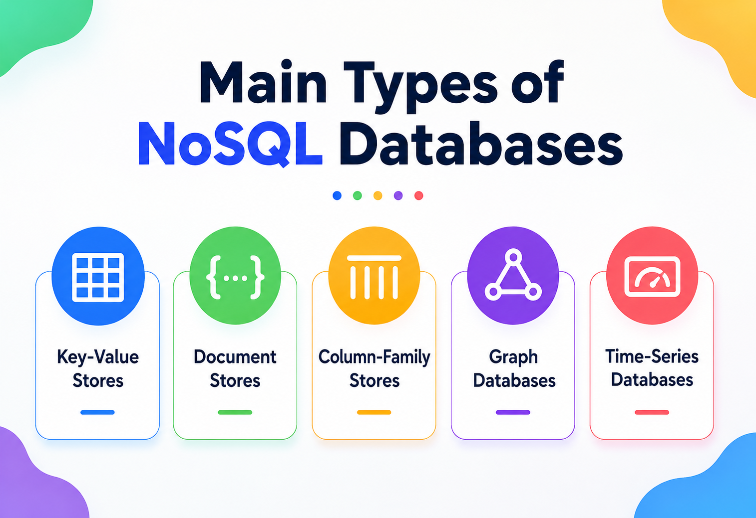
Almost every NoSQL database on the market fits into one of four core families, based on how it structures and models data. Some modern “multi-model” databases blend more than one of these, but understanding the four pure forms is the foundation for everything else.
The next four sections take each family in turn, using the same structure every time: what it is, why it exists, where it’s used, a real-world analogy, a beginner example, a working Java code sample, a production example from a well-known company, how it works internally, and the trade-offs to be aware of.
Key-Value Stores
The simplest, fastest, and often the most misunderstood NoSQL family.
Key-Value Stores
What it is: The simplest possible database model. Every piece of data is stored as a pair: a unique key (like a label) and a value (the actual data, which can be anything — a string, a number, a JSON blob, an image). You can only fetch data by its exact key — there’s no searching “inside” the value.
Why it exists: Sometimes you don’t need rich queries at all — you just need blazing-fast lookups, like “get me the shopping cart for user #4471, right now.” Stripping away everything except a key and a value lets these systems be extremely fast and simple.
A key-value store is exactly like a coat check counter at a theater. You hand over your coat and get a numbered ticket (the key). Later, you give the ticket back and instantly get your coat (the value) — the attendant doesn’t need to know anything about your coat’s color or size. They just match ticket numbers to coats on a shelf, as fast as possible.
Where it’s used
- Caching layers in front of slower databases (Redis, Memcached)
- Session storage for logged-in web users
- Shopping carts (Amazon’s original Dynamo use case)
- Real-time leaderboards and counters in games
- Feature flags and configuration lookups
Beginner example
Think of a simple phone contact list stored as key-value pairs:
"mom"      -> "+1-202-555-0143"
"pizza"    -> "+1-202-555-0199"
"dentist"  -> "+1-202-555-0170"
To find mom’s number, you look up the key "mom" directly — you never scan through every entry.
Software example (Java + Redis)
import redis.clients.jedis.Jedis;

public class CartCache {
    public static void main(String[] args) {
        // Connect to a local Redis server (a popular key-value store)
        try (Jedis redis = new Jedis("localhost", 6379)) {

            // WRITE: store a user's cart total under a key
            redis.set("cart:user:4471:total", "129.50");

            // Give the key a 30-minute expiry - carts should not live forever
            redis.expire("cart:user:4471:total", 1800);

            // READ: fetch it back by the exact key - this is O(1), instant
            String total = redis.get("cart:user:4471:total");
            System.out.println("Cart total: $" + total);
        }
    }
}
Explanation: set stores a value under a key, expire tells Redis to auto-delete it after a time limit (perfect for temporary session data), and get retrieves it instantly. There is no query language, no joins — just direct key lookups, which is why key-value stores are often the fastest NoSQL type.
Production example
Amazon built the original Dynamo system to power the shopping cart during massive Black Friday traffic spikes, prioritising “the cart must always accept an add-to-cart click” over perfect consistency. Twitter and GitHub use Redis to cache hot data (like a celebrity’s tweet timeline) so millions of reads never have to touch the slower primary database.
Internal working
Most key-value stores use a hash table (or hash index) under the hood — the same data structure you’d learn in an intro programming class. The key is run through a hash function that converts it into a memory address, so lookup is close to instant, regardless of how many million keys exist. Distributed key-value stores (like DynamoDB) additionally use consistent hashing to decide which physical server owns which key, and replicate that key to a few neighboring servers for durability.
Pros
- Extremely fast reads and writes.
- Very simple to reason about.
- Scales horizontally with almost no effort.
Cons
- No rich queries — you cannot ask “find all carts over $100” without scanning everything or building a separate index.
- No relationships between keys.
Document Databases
The family that most closely matches how developers already think about their objects in code.
Document Databases
What it is: A document database stores data as self-contained “documents” — usually in JSON-like format — instead of rows in a table. Each document can hold nested data (objects inside objects, lists inside objects) and different documents in the same collection don’t need identical fields.
Why it exists: A huge amount of real application data is naturally hierarchical — a blog post has comments, which have replies; a product has variants, which have prices. Cramming that into flat relational tables requires many separate tables and joins. A document database lets you store the whole object as one unit, matching how developers already think about their data in code.
A document database is like a filing cabinet full of individual folders. Each folder (document) can hold whatever papers are relevant to that one case — some folders are thick with attachments, some are thin — and you find a folder by flipping to its label (a unique ID), not by cross-referencing ten different cabinets.
Where it’s used
- Content management systems and blogging platforms
- Product catalogs (each product type has different attributes)
- User profiles with flexible, evolving fields
- Mobile app backends that store nested JSON straight from the app
Beginner example
A single “product” document might look like this:
{
  "_id": "p1001",
  "name": "Trail Running Shoe",
  "price": 89.99,
  "sizes": [8, 9, 10, 11],
  "reviews": [
    { "user": "amy", "stars": 5, "text": "Super comfortable!" },
    { "user": "raj", "stars": 4, "text": "Runs a little small." }
  ]
}
Notice the reviews live inside the product document — no separate “reviews” table and no join needed to display a product page.
Software example (Java + MongoDB)
import com.mongodb.client.*;
import org.bson.Document;
import java.util.Arrays;

public class ProductRepository {
    public static void main(String[] args) {
        try (MongoClient client = MongoClients.create("mongodb://localhost:27017")) {
            MongoDatabase db = client.getDatabase("shop");
            MongoCollection<Document> products = db.getCollection("products");

            // WRITE: insert a nested document in one call - no joins needed
            Document review  = new Document("user", "amy").append("stars", 5);
            Document product = new Document("_id", "p1001")
                    .append("name",   "Trail Running Shoe")
                    .append("price",  89.99)
                    .append("reviews", Arrays.asList(review));
            products.insertOne(product);

            // READ: query by a field, even one nested inside an array
            Document found = products.find(
                    new Document("reviews.stars", 5)
            ).first();

            System.out.println("Found product: " + found.getString("name"));
        }
    }
}
Explanation: The whole product, including its reviews, is written as one document in one operation — this is called an atomic write at the document level. The query on reviews.stars shows that document databases can still search inside nested fields, unlike plain key-value stores.
Production example
eBay and Forbes use MongoDB-family document databases to serve dynamic product and article pages. Uber historically used document-style storage (via Schemaless, built on MySQL, and later other systems) for ride and trip records with rapidly evolving structure.
Internal working
Documents are typically stored as BSON (Binary JSON) on disk for speed, grouped into “collections.” Databases build secondary indexes (often B-trees, the same balanced tree structure used in relational databases) on frequently-queried fields so lookups don’t require scanning every document. Sharding splits a huge collection across servers using a shard key — for example, splitting products by category so “shoes” and “electronics” queries hit different physical machines.
Pros
- Matches how developers think in code (objects).
- Flexible schema.
- Good read performance for whole-object reads.
- Supports rich queries and indexes.
Cons
- Joins across documents are awkward or slow — you either denormalise / duplicate data, or do multiple queries in application code.
- Large deeply-nested documents can get unwieldy.
Column-Family (Wide-Column) Stores
Built for the moments when you don’t just have “a lot of data” — you have web-scale data.
Column-Family (Wide-Column) Stores
What it is: Instead of storing data row-by-row like a relational table, column-family stores group and physically store data by column. Rows are identified by a row key, and each row can have a huge, sparse, and different set of columns, organised into groups called “column families.”
Why it exists: When you need to write and read massive volumes of data (billions of rows, potentially millions of columns) — like sensor readings, time-series logs, or search indexes — reading only the specific columns you need, without touching unrelated columns, is far faster. Google built Bigtable for exactly this reason, to index the entire web.
Imagine a giant spreadsheet where every row can be a completely different shape — one row might have 5 filled-in cells, another might have 5,000 — and the sheet is stored not by reading across a row, but by filing all the values of one column together, like sorting mail by which mailbox it goes to rather than by which mail carrier delivered it. If you only need “Column: temperature,” you can grab exactly that, without touching humidity, pressure, or any other column.
Where it’s used
- Time-series data — IoT sensor logs, stock market ticks, server metrics
- Messaging systems that need extremely high write throughput
- Recommendation and personalisation data at massive scale
- Search engine indexing (Bigtable’s original purpose at Google)
Beginner example
A column-family layout for sensor readings might look like this conceptually:
Row Key: "sensor-42"
  ColumnFamily "readings":
      2026-07-17T09:00 -> 21.4
      2026-07-17T09:05 -> 21.6
      2026-07-17T09:10 -> 21.3
  ColumnFamily "meta":
      location -> "Warehouse B"
      unit     -> "Celsius"
Each row key (“sensor-42”) can have a different, growing set of timestamp columns — some sensors might report every minute, others every hour, and that’s perfectly fine.
Software example (Java + Cassandra)
import com.datastax.oss.driver.api.core.CqlSession;
import com.datastax.oss.driver.api.core.cql.ResultSet;
import com.datastax.oss.driver.api.core.cql.Row;

public class SensorReadingsRepo {
    public static void main(String[] args) {
        try (CqlSession session = CqlSession.builder().build()) {

            // WRITE: append a new reading - Cassandra is optimized for fast writes
            session.execute(
                "INSERT INTO iot.readings (sensor_id, reading_time, value) " +
                "VALUES ('sensor-42', toTimestamp(now()), 21.4)"
            );

            // READ: fetch the most recent readings for one sensor, already sorted
            ResultSet rs = session.execute(
                "SELECT reading_time, value FROM iot.readings " +
                "WHERE sensor_id = 'sensor-42' ORDER BY reading_time DESC LIMIT 10"
            );

            for (Row row : rs) {
                System.out.println(row.getInstant("reading_time") + " -> " + row.getDouble("value"));
            }
        }
    }
}
Explanation: The table is designed around the row key (sensor_id) that will be used to fetch data, and Cassandra physically stores each sensor’s readings clustered together on disk, sorted by time — so “give me the last 10 readings for sensor-42” is a fast sequential read, not a search through billions of unrelated rows.
Production example
Netflix uses Cassandra to track viewing history and personalisation data across hundreds of millions of users, needing extremely high write throughput with no single point of failure. Apple reportedly runs one of the largest Cassandra deployments in the world across tens of thousands of nodes. Google continues to use Bigtable to power Search, Maps, and Gmail infrastructure.
Internal working
Column-family stores are built around a data structure called an LSM-Tree (Log-Structured Merge-Tree). New writes go first into an in-memory structure (a “memtable”), and are also appended to an on-disk write-log for durability. When the memtable fills up, it’s flushed to disk as an immutable file (an “SSTable”). Over time, a background process called compaction merges these SSTables together, discarding old or deleted data. This design makes writes extremely fast (just append, no need to find-and-update in place), which is why column-family stores excel at massive write throughput.
Pros
- Extremely high write throughput.
- Scales to petabytes across thousands of nodes.
- Efficient for sparse, wide data and time-series patterns.
Cons
- Query patterns must be designed in advance around the row key — you can’t easily ask arbitrary ad-hoc questions.
- Reads can be slower if data isn’t compacted well.
- Steeper learning curve for data modeling.
Graph Databases
When the interesting thing about your data is not the rows themselves but the connections between them.
Graph Databases
What it is: A graph database stores data as nodes (things, like people or products) and edges (relationships between things, like “follows” or “purchased”). Both nodes and edges can hold properties (extra data). The relationships themselves are treated as first-class citizens, stored and indexed directly, rather than computed on the fly through joins.
Why it exists: Some data is fundamentally about connections — who knows whom, what product leads to what other purchase, which computer talks to which server. In a relational database, answering “friends of friends of friends who like hiking” requires multiple expensive joins that get slower with every extra “hop.” A graph database can walk from node to node almost instantly, because each node directly stores pointers to its connected edges.
A graph database is like a corkboard covered in photos of people, connected with pieces of string to show who is friends with whom, or who reports to whom at work. To find out who Amy’s friends’ friends are, you just physically follow the strings from photo to photo — you don’t need to reread the whole corkboard from scratch.
Where it’s used
- Social networks (friend / follow graphs)
- Recommendation engines (“customers who bought X also bought Y”)
- Fraud detection (spotting unusual patterns of connected accounts and transactions)
- Network and IT infrastructure mapping
- Knowledge graphs powering search engines and AI assistants
Beginner example
A tiny social graph, described in plain words:
(Amy) -FOLLOWS-> (Raj)
(Raj) -FOLLOWS-> (Mia)
(Amy) -LIKES->   (Photo #17)
(Raj) -POSTED->  (Photo #17)
To answer “does Amy indirectly follow Mia through someone?”, the database simply walks: Amy → Raj → Mia. That’s a 2-hop traversal, and it stays fast even in a graph with billions of nodes, because each node already knows its direct neighbors.
Software example (Java + Neo4j)
import org.neo4j.driver.*;

public class FriendGraph {
    public static void main(String[] args) {
        try (Driver driver = GraphDatabase.driver(
                "bolt://localhost:7687", AuthTokens.basic("neo4j", "password"));
             Session session = driver.session()) {

            // WRITE: create two people and a FOLLOWS relationship between them
            session.run(
                "MERGE (a:Person {name:'Amy'}) " +
                "MERGE (r:Person {name:'Raj'}) " +
                "MERGE (a)-[:FOLLOWS]->(r)"
            );

            // READ: find friends-of-friends, 2 hops away - a graph's specialty
            Result result = session.run(
                "MATCH (a:Person {name:'Amy'})-[:FOLLOWS*2]->(fof) " +
                "RETURN DISTINCT fof.name"
            );

            while (result.hasNext()) {
                System.out.println("Friend of a friend: "
                    + result.next().get("fof.name").asString());
            }
        }
    }
}
Explanation: The query language (Cypher) directly expresses “follow this relationship type, two hops out” — something that would require multiple nested SQL joins, and get progressively slower with each extra hop in a relational database, but stays efficient here because each node stores direct references to its edges.
Production example
LinkedIn built its own large-scale graph engine to power “People You May Know” and connection paths (“2nd-degree connection”). PayPal uses graph databases to detect fraud rings by spotting unusual clusters of connected accounts and transactions in real time. eBay uses graph technology for product recommendations.
Internal working
Graph databases use a technique called index-free adjacency: each node physically stores direct pointers to its adjacent edges, so traversing a relationship is a constant-time pointer lookup, not a search through an index. This is fundamentally different from a relational join, where the database must search an index for every matching row at every step. This is also why deep traversals (many hops) tend to be a graph database’s biggest strength compared to every other NoSQL type.
Pros
- Extremely fast for relationship-heavy queries and deep traversals.
- Intuitive data model for connected data.
- Great for pattern-finding (fraud, recommendations).
Cons
- Not ideal for simple aggregate queries over huge unconnected datasets.
- Horizontal scaling (sharding a graph across machines while keeping traversals fast) is technically harder than the other three types.
Other NoSQL Flavors Worth Knowing
Beyond the four core families, a few specialised categories come up often enough in interviews and real systems that they deserve a quick mention.
Search engines
Elasticsearch, OpenSearch. Optimised for full-text search and relevance ranking, built on an inverted index (mapping words back to the documents that contain them) — similar to the index at the back of a textbook.
Time-series databases
InfluxDB, TimescaleDB. Purpose-built for data points ordered by time, like metrics and sensor data — conceptually related to column-family stores but with extra time-based optimisations.
Multi-model databases
ArangoDB, Cosmos DB, Fauna. Support more than one data model (document, graph, key-value) within a single engine, useful when a team doesn’t want to run and operate several different database systems.
Object & wide-column hybrids
Some cloud databases (like Amazon DynamoDB) blur the line between key-value and document stores, letting you attach rich attribute maps to a primary key while still guaranteeing single-digit-millisecond lookups.
These are important tools, but the four core families — key-value, document, column-family, and graph — remain the foundation you’ll be asked about in system design interviews and will reach for most often in production.
Internal Working — How Data Actually Gets Written and Read
Even though each NoSQL family stores data differently, most distributed NoSQL systems share a common internal playbook for handling a write.
10.1 · Step-by-step breakdown
Client sends the write
The application sends a write request to any node in the cluster; that node becomes the coordinator for this particular request.
Consistent hashing picks the owners
The coordinator applies a hash function to the key to figure out which nodes are responsible for storing that key (usually N nodes, where N is the replication factor).
Fan-out to replicas
The coordinator forwards the write in parallel to all N replicas.
Wait for quorum
Once W replicas acknowledge the write, the coordinator returns success to the client, even if some replicas haven’t yet responded.
Repair & catch up
Slower or temporarily-unreachable replicas eventually receive the write through background repair mechanisms (like hinted handoff and read repair).
Quorum, explained simply: If a piece of data is replicated to 3 servers (N=3), the database can require, say, 2 of them to confirm a write (W=2) and 2 to confirm a read (R=2) before calling it successful. Whenever R + W > N, you are mathematically guaranteed the read will see the latest write — this is how many NoSQL databases let you dial consistency up or down per operation.
Imagine 3 friends each keep a copy of your family’s shared calendar. If you require at least 2 out of 3 to agree before trusting what’s on the calendar (for both adding and checking events), you’ll always catch the latest update — because any 2-out-of-3 group and any other 2-out-of-3 group must overlap by at least one person.
Data Flow & Lifecycle — A Complete Example
Let’s trace one concrete request end-to-end: a user adds an item to their shopping cart on an e-commerce site backed by a key-value store, with a document database for the product catalog.
11.1 · Walkthrough
User clicks “Add to cart”
The browser sends
POST /cart/addwith the product ID and quantity to the application server.Fetch the product
The app looks up the product in MongoDB by
_id, retrieving the nested product document (price, name, images, options).Load the current cart
The app reads the current cart from Redis using the key
cart:user:4471. If none exists, it starts from an empty cart object in memory.Merge and persist
The new item is merged into the cart, and the whole updated cart is written back to Redis with a fresh 30-minute expiry.
Respond
The server returns
200 OKwith the updated cart total to the browser.
This is a real-world illustration of polyglot persistence: no single database type was “the best” choice for the whole app — each type was picked for the specific access pattern it’s best at.
Advantages, Disadvantages & Trade-offs
Every architectural choice has two sides. Here they are laid out honestly — family by family, and then NoSQL as a whole vs. relational databases.
12.1 · Family-by-family cheat sheet
| Type | Best at | Weak at | CAP leaning (typical default) |
|---|---|---|---|
| Key-Value | Ultra-fast simple lookups, caching, sessions | Complex queries, relationships | AP (e.g., DynamoDB, Redis Cluster) |
| Document | Flexible, nested, evolving data; whole-object reads | Multi-document joins/transactions at scale | Configurable; CP-leaning by default in MongoDB |
| Column-Family | Massive write throughput, time-series, wide sparse data | Ad-hoc queries not matching the row key design | AP (e.g., Cassandra), CP (e.g., HBase) |
| Graph | Deep relationship traversal, pattern discovery | Simple bulk aggregate scans, easy horizontal sharding | Typically CP (e.g., Neo4j in single-cluster mode) |
12.2 · General NoSQL vs. relational databases
| Dimension | Relational (SQL) | NoSQL (general) |
|---|---|---|
| Schema | Fixed, enforced upfront | Flexible, can evolve per record |
| Scaling | Primarily vertical (bigger machine) | Primarily horizontal (more machines) |
| Transactions | Strong ACID across many tables | Often limited to a single document/row; multi-record transactions vary by product |
| Query power | Very expressive (SQL joins, aggregates) | Simpler, purpose-built query patterns |
| Consistency | Strong by default | Often eventual, tunable |
| Best for | Structured data with complex relationships and strict correctness needs (banking, inventory) | Massive scale, flexible / rapidly-changing data, high availability needs |
“NoSQL is always faster than SQL.” Not true. NoSQL databases are faster for the specific access patterns they were designed for. A well-indexed relational query can easily outperform a poorly modeled NoSQL query. Speed comes from matching the data model to the access pattern — not from the label “NoSQL” itself.
Performance & Scalability
NoSQL databases weren’t just designed to handle big data — they were designed to make scaling predictable. Here are the techniques that make that possible.
13.1 · Partitioning strategies
- Range partitioning: Data is split by ranges of the key (e.g., users A–M on server 1, N–Z on server 2). Simple, but can create “hot spots” if data isn’t evenly distributed.
- Hash partitioning: A hash function spreads keys evenly across servers, avoiding hot spots, but makes range queries (like “all users starting with A”) harder, since related keys land on random servers.
- Consistent hashing: (explained earlier) minimises data movement when servers are added or removed — critical for systems that must scale up and down without massive, disruptive rebalancing.
13.2 · Read / write throughput tricks
- Denormalization: Deliberately duplicating data (e.g., storing a user’s name inside every one of their comments) to avoid expensive joins at read time. This is common and accepted in NoSQL, unlike in relational design.
- Caching layers: Placing a key-value store like Redis in front of a slower database to absorb repeated reads.
- Write batching: Grouping many small writes into fewer, larger operations to reduce network and disk overhead.
13.3 · Big-O intuition for common operations
| Operation | Key-Value | Document (indexed) | Column-Family | Graph (traversal) |
|---|---|---|---|---|
| Point lookup by key / ID | O(1) | O(log n) | O(1)–O(log n) | O(1) |
| Range scan | Not supported natively | O(log n + k) | O(log n + k) | N/A |
| k-hop relationship traversal | Not supported | Expensive, needs multiple queries | Not supported | O(k) with index-free adjacency |
(n = total records, k = number of results / hops. These are practical approximations, not formal proofs — actual performance depends heavily on indexing and data modeling.)
High Availability & Reliability
Distributed NoSQL databases were born in an environment where servers will fail — the design assumes it, and the tooling reflects it.
14.1 · Replication strategies
- Leader-follower (primary-replica): One node accepts writes and streams changes to read-only followers. Simple, but the leader can become a bottleneck or single point of failure until a new leader is elected.
- Leaderless (multi-master): Any replica can accept a write (used by Cassandra and DynamoDB). More available, but requires conflict resolution when two replicas get different writes for the same key at nearly the same time.
14.2 · Conflict resolution
When two replicas disagree (e.g., two people updated the same key while a network partition was happening), the database needs a rule to reconcile them:
- Last-Write-Wins (LWW): The write with the newest timestamp wins. Simple, but can silently lose data.
- Vector clocks: Track the causal history of updates across replicas, so the system can detect true conflicts (rather than just “newer”) and, in some designs, let the application decide how to merge them.
- CRDTs (Conflict-free Replicated Data Types): Special data structures (like counters or sets) mathematically designed so that merging two divergent copies always produces a consistent result, with no manual conflict resolution needed.
14.3 · Failure detection & recovery
Distributed NoSQL databases constantly send small heartbeat messages between nodes (a “gossip protocol” in Cassandra-style systems) to detect failures quickly. When a node is marked as down, the cluster automatically routes its traffic to healthy replicas, and once it recovers, a repair process (like Cassandra’s “hinted handoff” and “read repair”) catches it back up with any writes it missed.
Security
The looser schema and richer feature set of NoSQL databases doesn’t mean looser security — if anything, it demands more discipline.
- Authentication & authorization: Modern NoSQL databases support role-based access control (RBAC) — e.g., a reporting service might get read-only access, while the application server gets read-write access to specific collections/tables only.
- Encryption in transit: TLS / SSL should always be enabled between application and database, and between cluster nodes themselves.
- Encryption at rest: Data files on disk should be encrypted, so a stolen disk doesn’t expose raw data.
- Network isolation: Databases should sit inside private subnets / VPCs, never directly exposed to the public internet — a mistake that has caused several major exposed-MongoDB-instance data leaks in the past.
- Injection risks: Even NoSQL databases can suffer injection attacks (e.g., “NoSQL injection” through poorly sanitised JSON query operators in MongoDB). Always validate and parameterise user input rather than concatenating raw strings into queries.
- Auditing: Logging who accessed or changed what data is essential for compliance (GDPR, HIPAA, PCI-DSS) and for catching suspicious activity.
Leaving a NoSQL database’s default port open to the internet with no authentication — this has caused real, large-scale data breaches. Always enable authentication and restrict network access, even for “internal” databases.
Monitoring, Logging & Metrics
Whichever NoSQL database you run in production, track these categories of metrics.
- Latency: p50, p95, and p99 read / write latency — averages hide the painful outliers that real users feel.
- Throughput: Operations per second, to catch traffic spikes or degraded capacity.
- Error rates: Timeouts, connection failures, and rejected writes (often due to overloaded nodes).
- Replication lag: How far behind a replica is from the primary — critical for spotting eventual-consistency risk before users notice stale reads.
- Resource usage: CPU, memory, disk I/O, and (for LSM-tree databases) compaction backlog, which can silently degrade read performance if ignored.
- Cluster health: Node up/down status, number of healthy replicas per shard.
Common tooling: Prometheus + Grafana dashboards, along with database-specific tools (MongoDB Atlas monitoring, DataStax OpsCenter for Cassandra, Neo4j’s built-in metrics). Distributed tracing (OpenTelemetry, Jaeger) helps pinpoint whether a slow user request was actually caused by a slow database call, a slow cache miss, or something else in the chain.
Deployment & Cloud
Very few teams today run NoSQL databases entirely by hand. Here are the common deployment options and their trade-offs.
- Fully managed cloud services: Amazon DynamoDB, Google Cloud Firestore / Bigtable, Azure Cosmos DB, MongoDB Atlas, Neo4j Aura. The cloud provider handles patching, backups, scaling, and failover — you mostly configure capacity and access.
- Self-managed on Kubernetes: Using Helm charts or operators (e.g., the Cassandra Operator, MongoDB Community Operator) to run a database cluster inside your own Kubernetes environment, trading operational effort for more control and often lower cost at scale.
- Multi-region deployment: Many NoSQL databases support active-active replication across regions, so users on different continents read / write to a nearby copy, improving latency and disaster recovery — at the cost of embracing eventual consistency between regions.
Managed NoSQL services often charge by provisioned throughput (e.g., DynamoDB’s read/write capacity units) or by actual usage (on-demand mode). For spiky, unpredictable traffic, on-demand pricing avoids paying for idle capacity; for stable, predictable traffic, provisioned capacity is usually cheaper.
Databases, Caching, Load Balancing, APIs & Microservices
NoSQL databases rarely operate alone — they sit inside a larger system alongside caches, load balancers, and services.
Key ideas: each microservice typically owns its own database (avoiding tight coupling between services), a load balancer spreads incoming API requests across multiple stateless application instances, and a caching layer absorbs repeat reads before they ever reach the primary database. NoSQL databases pair naturally with REST and gRPC APIs because their document / JSON-like data often maps directly onto API request and response bodies with little translation needed.
This ecosystem view also explains why so many teams end up mixing multiple NoSQL types in one product: the catalog service is document-shaped, the cart service is key-value-shaped, the recommendation service is graph-shaped — and forcing all three into one database technology would leave real performance and clarity on the table.
Design Patterns & Anti-patterns
Every real production NoSQL system is built from a small library of good habits — and a careful avoidance of a few common traps.
19.1 · Good patterns
- Query-first modeling: In NoSQL, you design your data model around the exact queries your application needs to run — the opposite order from relational design, where you normalise data first and write queries later.
- Denormalization for read speed: Duplicating small pieces of data (like a username) across many documents to avoid joins, accepting the small cost of updating duplicates when that data rarely changes.
- Time-bucketing: In column-family stores, grouping time-series data into buckets (e.g., one row per sensor per day) to keep individual rows from growing unbounded.
- Polyglot persistence: Using different NoSQL (and SQL) types for different services or features within the same overall system, rather than forcing one database to do everything.
19.2 · Anti-patterns to avoid
Anti-pattern 1 — document DB as a relational DB
Over-normalising data into many small linked collections, then doing the equivalent of joins in application code for every request — this throws away the main advantage of the document model.
Anti-pattern 2 — unbounded arrays / rows
Letting a document’s array (like “comments”) or a column-family row grow forever without limits — eventually a single document / row becomes too large to read or write efficiently.
Anti-pattern 3 — ignoring the shard / partition key
Choosing a bad partition key (e.g., a key with very few unique values, like “country” for a mostly-single-country app) creates “hot partitions” that overload one server while others sit idle.
Anti-pattern 4 — a graph DB for everything
Graph databases shine for relationship-heavy queries but are a poor fit for simple bulk reporting / aggregation over huge unrelated datasets.
Best Practices & Common Mistakes
A distilled checklist you can print out and stick above the whiteboard.
Design for your access patterns first
Ask “what will I query?” before “how should I structure this?” — not the other way around.
Choose partition / shard keys with high cardinality
Many unique values and even access distribution avoid hot spots that overload a single node.
Set sensible TTLs on temporary data
Sessions, caches, and short-lived tokens should expire automatically so old data doesn’t silently pile up forever.
Monitor replication lag & consistency level
Know what consistency level your application actually needs per operation — not every read needs the strongest, slowest setting.
Automate backups and regularly test restores
A backup you’ve never restored from is not a real backup.
Avoid “one database to rule them all” thinking
It’s normal and often correct to use two or three different NoSQL types (plus a relational database) inside one system.
Don’t skip capacity planning
Know your expected read / write volume and growth rate before choosing configuration, especially on managed services billed by throughput.
Real-World & Industry Examples
These aren’t textbook diagrams — they’re the actual patterns running behind services you use every day.
Netflix · Cassandra (Column-Family)
Stores viewing history and personalisation signals across hundreds of millions of users with extremely high write throughput and no single point of failure.
Amazon · DynamoDB (Key-Value / Document)
Powers shopping carts and order data with single-digit-millisecond latency at massive scale, prioritising availability during peak sales events.
Facebook / Meta · Graph technology
The social graph (friends, pages, groups) is fundamentally relationship data — one of the earliest and largest real-world uses of graph-style thinking at scale.
LinkedIn · Graph engine
Powers “People You May Know” and connection-degree calculations (1st, 2nd, 3rd-degree connections) using fast relationship traversal.
Uber · Document-style storage
Stores rapidly evolving trip and rider data where the schema changes often as new features ship.
PayPal · Graph database
Detects fraud rings by finding unusual clusters of connected accounts and transactions in near real time.
Google · Bigtable (Column-Family)
Backs Search, Maps, and Gmail, storing and retrieving specific columns out of enormous, sparse datasets efficiently.
Twitter / X, GitHub · Redis (Key-Value)
Caches hot data — trending timelines, session tokens — in front of slower primary databases to absorb massive read volume.
Frequently Asked Questions
The questions engineers most often ask when they first meet NoSQL — and the honest, non-marketing answers.
Is NoSQL going to replace SQL databases?
No. They solve different problems and are commonly used together in the same system (polyglot persistence). Relational databases remain the best choice when you need strong, multi-table transactional correctness.
Which NoSQL type should I learn first?
Document databases (like MongoDB) are usually the friendliest starting point for developers coming from JSON-based web APIs, followed by key-value stores (like Redis) for caching concepts.
Can NoSQL databases do transactions?
Many now support transactions, but with different scopes and guarantees than relational databases. MongoDB, for example, added multi-document ACID transactions in later versions, but they’re used sparingly since they work against the model’s natural strengths.
Is eventual consistency dangerous?
Not inherently — it’s a deliberate trade-off. It’s dangerous only when used for data that truly needs strong consistency (like account balances) without understanding the risk. For “like” counts or activity feeds, it’s usually a non-issue.
How do I decide between document and column-family for structured data?
If your access pattern is “fetch one rich, nested object by ID” — document. If it’s “write huge volumes of narrow, time-ordered data and read ranges of it by a known key” — column-family.
Do NoSQL databases support SQL-like query languages?
Some do, to ease the learning curve — Cassandra’s CQL looks SQL-like, and many document databases offer SQL-style query layers on top of their native APIs — but the underlying data model and capabilities remain different from a relational database.
Note: this is general educational information about database technology, not medical, legal, or safety guidance.
Summary & Key Takeaways
If you remember only a handful of ideas from this tutorial, make it these.
Key takeaways
- NoSQL databases emerged to solve real problems relational databases struggled with: massive scale, flexible / rapidly-evolving data, and high availability across distributed systems.
- There are four core NoSQL families: Key-Value (fastest, simplest lookups), Document (flexible nested objects), Column-Family (massive write throughput, wide sparse data), and Graph (relationship-heavy traversal).
- The CAP theorem explains the fundamental trade-off every distributed NoSQL database makes between consistency and availability during a network partition.
- Most NoSQL databases favor BASE over strict ACID, though many now offer tunable consistency and limited transaction support.
- Good NoSQL design starts from your application’s actual query patterns, not from abstract data-normalisation rules.
- Real production systems almost always use several database types together — this is normal, expected, and called polyglot persistence.
- Operational concerns — replication, partitioning, monitoring, security, and disaster recovery — matter just as much as picking the “right” database type.
There is no single “best” NoSQL database — only the best database for a specific job. The real skill isn’t memorising which company uses which product; it’s learning to look at an access pattern and ask, “does this need fast key lookups, flexible nested documents, massive write throughput, or deep relationship traversal?” — and letting that question guide your choice.