What Is a Graph Database Used For?
From “what even is a node” to how Netflix, LinkedIn, and Amazon Neptune use graphs at scale — explained with plain-English analogies, real diagrams, and production-grade Java examples. Nodes are things. Edges are relationships. Index-free adjacency is what makes deep relationship queries stay fast no matter how big the graph grows.
A graph database is a purpose-built engine for storing things (nodes), the relationships between them (edges), and the small pieces of data attached to either (properties). This guide walks 19 sections from the 1736 origins of graph theory through the modern property graph model, the layered anatomy of a graph engine, the index-free adjacency trick that keeps traversals fast at any scale, a Java example against Neo4j, replication with Raft consensus, deployment on managed services like Amazon Neptune and Neo4j Aura, and case studies from Netflix, LinkedIn, Amazon, Uber, and Google's Knowledge Graph.
Introduction & History
Dots and lines — from Euler's Königsberg bridges in 1736 to modern engines like Neo4j, Neptune, and JanusGraph running at web scale.
Imagine you have a giant box of photographs of your family. Each photo shows one or two people. Now imagine someone asks you: “How is your grandmother's cousin's son related to you?” If your photos are just piled in a box, answering that question means digging through hundreds of pictures, trying to remember who is connected to whom. But if instead you had drawn a family tree — a diagram with names connected by lines showing “parent of,” “married to,” “sibling of” — you could trace the answer in seconds just by following the lines.
That family tree is, in essence, a graph. And a graph database is a computer system built specifically to store information the way that family tree stores it: as things (people, places, products, accounts) connected to each other by relationships (parent-of, bought, follows, works-at). Instead of hiding relationships inside rows and columns like traditional databases do, a graph database makes relationships the star of the show.
1.1 · WHY “GRAPH”? A QUICK WORD ON THE NAME
In everyday language, “graph” usually means a bar chart or a line chart plotting numbers. In computer science, “graph” means something different — it comes from a branch of mathematics called graph theory, founded in 1736 by the Swiss mathematician Leonhard Euler. Euler was trying to solve a puzzle in the city of Königsberg: the city had seven bridges connecting different parts of land, and people wondered if you could take a walk that crossed every bridge exactly once and returned to the start. Euler represented the land masses as dots and the bridges as lines connecting the dots. That simple idea — dots and lines representing things and their connections — is the foundation of every graph database that exists today, almost 300 years later.
Simple analogy
Think of a graph database as a giant social map pinned to a wall, with photographs (the “things”) connected by pieces of string (the “relationships”). You can literally trace a string with your finger from one photo to another to see how they're connected. A graph database lets a computer do that tracing instantly, even across millions of photos and billions of strings.
1.2 · A SHORT HISTORY
For most of computing history, the dominant way to store data was the relational database — think spreadsheets with rows and columns, joined together with keys (MySQL, PostgreSQL, Oracle). This model, introduced by Edgar F. Codd in 1970, was extremely successful because most early business data — customers, orders, invoices — fit neatly into tables.
But by the early 2000s, the internet had created a new kind of data problem: social networks, recommendation engines, and fraud detection systems all needed to understand how things are connected, not just what the things are. Answering “who are my friend's friends” in a relational database requires expensive operations called joins, and those joins get slower and slower as the network grows. Engineers needed a database designed around connections from day one.
This led to the rise of dedicated graph databases: Neo4j (first released in 2007) became the most widely adopted; Amazon Neptune, launched in 2017, brought managed graph databases to the cloud; Microsoft's Azure Cosmos DB added a graph API (Gremlin); and open-source engines like JanusGraph, ArangoDB, and TigerGraph emerged to handle different scales and workloads. Today, graph databases are considered one of the core categories of the “NoSQL” (Not Only SQL) database movement, alongside document, key-value, and column-family databases.
The Problem & Motivation
Why “friend-of-a-friend-of-a-friend” falls off a cliff in a relational database — and why relationship-first storage was inevitable.
To understand why graph databases exist, it helps to first understand what goes wrong when we try to store highly connected data in a traditional table-based (relational) database.
2.1 · THE “JOIN EXPLOSION” PROBLEM
Suppose you run a small social network. You have a table of users and a table called friendships that stores pairs of user IDs who are friends. If someone asks “show me my friends,” that's one simple join — fast and easy. But if they ask “show me my friends' friends' friends who are not already my friends” (a very normal question for a “people you may know” feature), you now need to join the friendships table to itself three or four times.
Each of those joins is expensive. The database has to scan large chunks of the table, match rows, and combine them, and the cost multiplies at every additional “hop” in the relationship chain. This is sometimes called join explosion: performance doesn't degrade gently, it falls off a cliff as you ask about deeper and more complex relationships.
In a relational database, a 2-hop query (friends-of-friends) might take milliseconds. A 4-hop query on the same data can take minutes or simply time out, because the number of possible paths to check grows exponentially, not linearly. This is exactly the kind of query graph databases were built to make fast.
2.2 · REAL QUESTIONS THAT ARE HARD FOR TRADITIONAL DATABASES
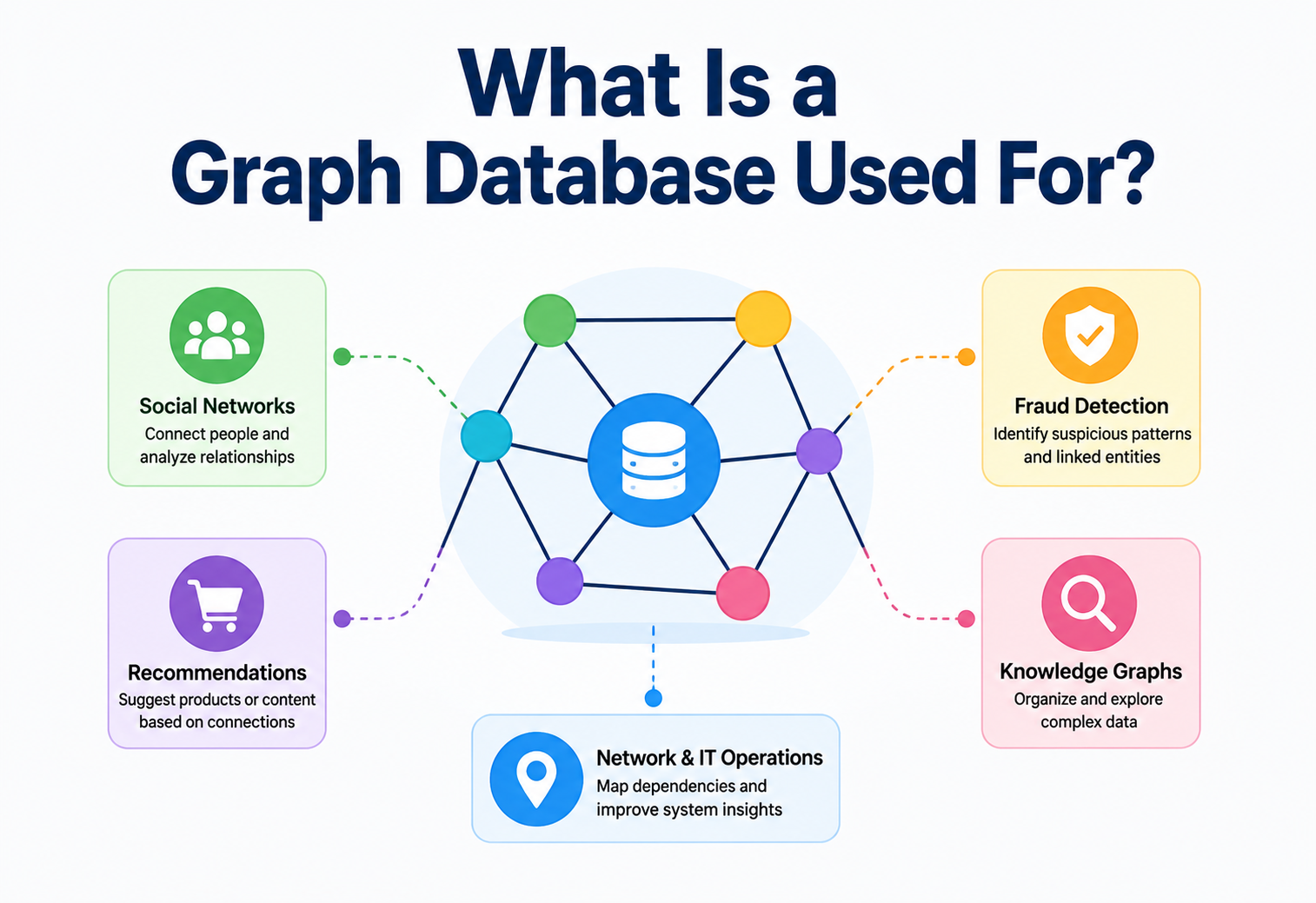
- Fraud detection: “Does this new bank account share a phone number, address, or device fingerprint with any account previously flagged for fraud, even indirectly through 3 other accounts?”
- Recommendation engines: “What products did people similar to me buy, where 'similar' means they bought at least 3 of the same items I did?”
- Social networks: “What's the shortest chain of connections between me and this stranger?” (This is the famous “six degrees of separation” idea.)
- Network & IT operations: “If this server goes down, which other services and customers are affected, considering all the dependencies?”
- Knowledge graphs: “What movies did an actor appear in that were directed by someone who also directed a movie starring a different specific actor?”
All of these questions share a pattern: the answer depends on traversing (walking across) a chain of relationships, and the number of hops is not known in advance. Relational databases are optimized for looking things up by known keys and doing a small, fixed number of joins — not for open-ended relationship traversal. Graph databases were purpose-built to make this class of question fast and natural to express.
Beginner example
Imagine trying to find out if you can get from your house to your friend's house using only roads shown on a paper map, but the map is actually a giant spreadsheet listing every road as a separate row with a “from street” and “to street” column, in no particular order, spread across 500 pages. You'd have to keep flipping pages, cross-referencing street names. A graph database is like having the actual folded paper map instead — you can trace the route with your finger.
Core Concepts
The vocabulary you'll use forever: node, edge, direction, property, label, path, traversal — plus the property graph vs RDF model split.
Let's build up the vocabulary of graph databases one term at a time. Each term below is something you will see over and over again, so it's worth taking your time here.
Node (or Vertex)
What it is: A node (sometimes called a “vertex,” plural “vertices”) represents one single “thing” — a person, a product, a city, a bank account, a movie. It is the “dot” in our dots-and-lines picture.
Why it exists: Every piece of data needs a home. A node is the container that holds one real-world entity so it can be referred to and connected to other entities.
Where it's used: A user profile on a social app, a single product in a catalog, a single sensor in an IoT network — all of these become nodes.
Analogy
A node is like a single sticky note pinned to a corkboard. Each sticky note has a name written on it, like “Priya” or “iPhone 15” or “Delhi.”
Edge (or Relationship)
What it is: An edge is the “line” connecting two nodes. It represents how those two things relate to each other — for example, “Priya FOLLOWS Rahul” or “Rahul PURCHASED iPhone 15.”
Why it exists: Data on its own is boring; the interesting insight almost always comes from how pieces of data relate to each other. Edges make relationships a first-class citizen of the database, not an afterthought bolted on with foreign keys.
Where it's used: “Friend of,” “reports to,” “is a part of,” “is located in,” “bought,” “rated 5 stars” — any verb connecting two nouns can become an edge.
Analogy
If nodes are sticky notes, an edge is a piece of string connecting two sticky notes, often with a small label tied to the string describing the relationship, like “married to” or “manager of.”
Direction
Most graph databases give edges a direction — an arrow pointing from one node to another. “Priya FOLLOWS Rahul” is different from “Rahul FOLLOWS Priya,” just like following someone on Instagram doesn't mean they follow you back. Some relationships are naturally two-way (like “married to”), and most graph databases let you query in either direction even if the edge was stored with one direction, but the direction itself is still stored as metadata.
Property
What it is: A property is a small piece of extra information attached to a node or an edge, stored as a key-value pair. A “Person” node might have properties like name: "Priya", age: 29, city: "Delhi". An edge like PURCHASED might have a property date: "2026-03-14" or amount: 79999.
Why it exists: Not every detail about a thing deserves to become its own node. Properties let you attach lightweight facts directly to the node or edge they describe, without cluttering the graph with unnecessary connections.
In a movie recommendation graph, a RATED edge between a User node and a Movie node might carry a property stars: 4. This lets you ask, “Find movies rated 4 stars or higher by users who also liked the movies I liked” — the rating detail lives right on the connection itself, not in a separate table.
Label (or Type)
What it is: A label categorizes a node, similar to how a table name categorizes rows in a relational database. A node might be labeled Person, Product, or City. A node can even have multiple labels, e.g. Person and Employee at the same time.
Why it exists: Labels let the database (and the humans reading a query) quickly filter nodes by kind — “give me all Person nodes” — without scanning every single node in the graph.
3.1 · THE PROPERTY GRAPH MODEL
The combination of nodes, edges, labels, and properties is called the property graph model — the most widely used graph data model today (used by Neo4j, Amazon Neptune, JanusGraph, ArangoDB, and others). It's popular because it maps naturally to how humans already think and speak: “Priya (a Person) FOLLOWS (relationship) Rahul (a Person) since 2023 (property).”
3.2 · RDF: THE OTHER MAJOR GRAPH MODEL
There's a second, older graph model worth knowing about for interviews: the Resource Description Framework (RDF), which stores data as “triples” — subject, predicate, object — such as (Priya, follows, Rahul). RDF comes from the academic Semantic Web community and is used in knowledge graphs like Wikidata and DBpedia, queried using a language called SPARQL. RDF graphs are typically simpler (edges usually don't carry their own properties) but are excellent for representing formal, standardized knowledge that needs to be shared and reasoned over across organizations.
3.3 · SCHEMA — STRICT VS. FLEXIBLE
Relational databases require you to define a fixed schema (column names and types) up front, and changing it later usually means running a migration across the whole table. Most graph databases are schema-optional: you can add a brand-new label, a brand-new relationship type, or a brand-new property on a single node without touching anything else in the database. Some engines also support schema constraints on top of this flexibility — for example, forcing every Person node to have a unique email property — giving you the best of both worlds: flexibility where you want it, and guardrails where you need them.
Imagine your family tree diagram again. If you suddenly learn about a great-aunt nobody had mentioned before, you can just draw a new sticky note and a new string connecting her to the tree — you don't need to redraw the whole diagram or change how every other sticky note works. That's schema flexibility in action.
3.4 · A WORKED MINI-EXAMPLE — MODELING A SMALL E-COMMERCE GRAPH
Let's walk through designing a tiny graph step by step, the way an architect would on a whiteboard. Say we want to model customers, products, and orders for an online store.
Identify the “things” (nodes)
Customer, Product, Order, Category.
Identify the “verbs” (edges)
A Customer PLACED an Order. An Order CONTAINS a Product. A Product BELONGS_TO a Category. A Customer VIEWED a Product.
Attach properties
The PLACED edge might carry a
dateproperty. The CONTAINS edge might carry aquantityproperty. The Product node might carrypriceandname.Ask your real questions, and check the model supports them
“What products do customers who bought Product A also tend to buy?” becomes a simple 3-hop traversal: Customer → PLACED → Order → CONTAINS → Product, repeated for a starting product and its co-purchasers.
Notice that we deliberately modeled Order as its own node instead of a direct edge from Customer to Product. This is the “intermediate node pattern” covered later in the Design Patterns section — it lets us attach order-level details (like a shipping address) and avoids losing information that a direct edge couldn't hold.
Path
A path is a sequence of nodes connected by edges — essentially a route through the graph. “Priya FOLLOWS Rahul FOLLOWS Ankit” is a path of length 2 (two hops). Most graph queries are, underneath, searches for paths that match some pattern.
Traversal
A traversal is the act of walking from node to node along edges, usually to answer a question like “what's reachable from here” or “what's the shortest way to get there.” This is the graph database's bread and butter, and we'll dig into the algorithms behind it in the Advanced Topics section.
Architecture & Components
Query language on top · index-free adjacency storage below · indexes, transactions, cache, and cluster layer holding it all together.
A graph database is not just “a database that stores dots and lines” — it's a full system with layers, just like any other database. Let's walk through the major components.
4.1 · QUERY LANGUAGE / QUERY ENGINE
This is the layer you talk to. Popular graph query languages include:
- Cypher — used by Neo4j and adopted as the basis for the new ISO standard GQL (Graph Query Language), ratified in 2024. Cypher reads almost like ASCII art:
(a:Person)-[:FOLLOWS]->(b:Person)visually looks like a node, an arrow, and another node. - Gremlin — a graph traversal language from the Apache TinkerPop project, used by Amazon Neptune, JanusGraph, and CosmosDB. It's more like a pipeline of steps:
g.V().has('name','Priya').out('FOLLOWS'). - SPARQL — the query language for RDF triple stores.
The query engine parses your query, builds an execution plan (deciding the fastest order to walk the graph), and hands work to the storage engine below it.
4.2 · STORAGE ENGINE (INDEX-FREE ADJACENCY)
This is the layer that makes graph databases fundamentally different from relational databases, and we'll dedicate the entire next section to it. In short: each node physically stores direct pointers to its neighboring nodes and edges, so “who is this node connected to” is answered by following a memory pointer instead of searching an index.
4.3 · INDEXES
Even though relationships don't need indexes to be fast, you still need a way to find your starting node quickly — for example, “find the Person node with email = x@example.com.” Graph databases maintain traditional indexes (often B-trees or hash indexes) on node/edge properties for exactly this purpose.
4.4 · TRANSACTION MANAGER
Handles ACID guarantees (Atomicity, Consistency, Isolation, Durability) for operations that create, update, or delete nodes and edges, so that concurrent writes don't corrupt the graph.
4.5 · CACHE / BUFFER POOL
Frequently accessed nodes and edges are kept in memory, because graph traversals tend to revisit “hub” nodes (like a popular celebrity account) very often. A good cache dramatically speeds up traversal-heavy workloads.
4.6 · CLUSTER / REPLICATION LAYER
In production, graph databases run as a cluster of multiple machines for fault tolerance and read scalability, using a consensus protocol (such as Raft) to keep replicas in sync — more on this in the High Availability section.
Internal Working — Index-Free Adjacency
The single most important idea to understand about graph databases: neighbours are found by following a pointer, not by searching an index.
This is the single most important idea to understand about how graph databases achieve their speed, and it comes up constantly in interviews.
5.1 · HOW A RELATIONAL DATABASE FINDS “FRIENDS OF A FRIEND”
In a relational database, if you want to find all of Priya's friends, the database looks up Priya's ID in a friendships table using an index (usually a B-tree), which takes roughly O(log n) time — fast, but not free, and it gets slower with every additional hop because each hop requires another index lookup across a potentially huge table.
5.2 · HOW A GRAPH DATABASE DOES IT — POINTER-CHASING, NOT SEARCHING
A graph database stores each node with a small, direct list of pointers to its adjacent (neighboring) relationships — physically, like a linked list sitting right next to the node's data. This means that finding “who is Priya connected to” doesn't require searching an index at all: the database just follows the pointer already stored on the Priya node, the same way you'd follow a piece of string tied directly to a sticky note. This design is called index-free adjacency, and it means traversal cost depends only on how much of the graph you actually visit — not on the total size of the database.
Analogy
Searching an index is like looking up a person's address in a phone book (you flip pages, compare names alphabetically). Index-free adjacency is like already holding that person's hand — you don't need to look anything up to know who they're connected to; you just follow the grip.
5.3 · WHY THIS MATTERS FOR “DEEP” QUERIES
Because each hop is a constant-time pointer-follow rather than an index search, a graph database's performance for relationship queries stays roughly constant per hop, regardless of how many total nodes exist in the whole database. A relational database's join-based approach, by contrast, tends to get proportionally slower as the overall table grows, because each join re-scans or re-indexes a large candidate set.
| Hops (degree of separation) | Relational DB (joins) | Graph DB (index-free adjacency) |
|---|---|---|
| 1 hop | Fast | Fast |
| 2 hops | Noticeably slower | Still fast |
| 3-4 hops | Very slow / expensive | Fast |
| 5+ hops | Often impractical | Fast (bounded by nodes actually visited) |
5.4 · NATIVE VS. NON-NATIVE GRAPH STORAGE
Not all “graph databases” implement true index-free adjacency at the storage layer. Some products add a graph query layer on top of a different underlying storage engine (for example, a key-value or column store) — these are sometimes called non-native graph databases. Native graph databases like Neo4j store adjacency information directly in the physical file layout. This is a common interview distinction: “native” refers to the storage engine, not just the query language exposed to developers.
Data Flow & Lifecycle
Six steps from connection to committed result — plus a real Java example that would take a self-join and a NOT EXISTS in SQL.
Let's trace what actually happens, step by step, when your application talks to a graph database.
Connection
Your application opens a connection (often via a driver, such as the official Neo4j Java driver) to the graph database, typically over a binary protocol (Neo4j uses “Bolt”) for efficiency.
Query submission
The application sends a query written in Cypher, Gremlin, or SPARQL, often with parameters (e.g.,
$userId) so the query plan can be cached and reused safely across different inputs.Parsing & planning
The query engine parses the text into an internal representation, then builds an execution plan — deciding, for example, whether to start the traversal from the “Priya” node (if there's a good index on name) or from some other anchor point, and in what order to expand relationships.
Traversal execution
The engine begins walking the graph using index-free adjacency, applying filters (property conditions), and following edges according to the query pattern, gathering matching paths as it goes.
Result assembly
Matched nodes, edges, and properties are collected into a result set — a table of rows, a graph visualization, or raw JSON, depending on how the client asked for the data.
Transaction commit (for writes)
If the query created, updated, or deleted anything, the transaction manager writes the change to a durable transaction log first (write-ahead logging), then commits it, ensuring the database can recover to a consistent state even after a crash.
6.1 · A JAVA EXAMPLE — CONNECTING AND QUERYING NEO4J
Below is a minimal, production-style example using the official Neo4j Java driver to find Priya's friends-of-friends who she doesn't already follow.
import org.neo4j.driver.*;
import static org.neo4j.driver.Values.parameters;

public class FriendRecommender {

    public static void main(String[] args) {
        // 1. Create a driver (thread-safe, reuse across the app)
        try (Driver driver = GraphDatabase.driver(
                "neo4j://localhost:7687",
                AuthTokens.basic("neo4j", "password"))) {

            // 2. Open a session
            try (Session session = driver.session()) {

                String cypher =
                    "MATCH (me:Person {name: $name})-[:FOLLOWS]->()-[:FOLLOWS]->(fof:Person) " +
                    "WHERE NOT (me)-[:FOLLOWS]->(fof) AND me <> fof " +
                    "RETURN DISTINCT fof.name AS suggestion " +
                    "LIMIT 10";

                // 3. Run the query with a parameter (never string-concatenate input!)
                var result = session.run(cypher, parameters("name", "Priya"));

                // 4. Consume the results
                while (result.hasNext()) {
                    Record record = result.next();
                    System.out.println("Suggested: " + record.get("suggestion").asString());
                }
            }
        }
    }
}
This one query — a 2-hop traversal with a filter — would require a multi-way self-join and a NOT EXISTS subquery in SQL. In Cypher, it reads almost like a sentence: “match me, following someone, who follows a friend-of-friend, where I don't already follow them.”
Advantages, Disadvantages & Trade-offs
What graph databases are unbeatable at — and where a column store or a plain relational database will still eat their lunch.
7.1 · ADVANTAGES
| Advantage | Why it matters |
|---|---|
| Fast relationship traversal | Index-free adjacency keeps multi-hop queries fast regardless of overall database size. |
| Intuitive data modeling | The schema mirrors how humans naturally describe relationships (“X follows Y”), reducing the mental translation needed to design and query the database. |
| Schema flexibility | Most graph databases are schema-optional — you can add new node types, labels, or properties without a disruptive migration. |
| Powerful pattern matching | Queries can express complex shapes (triangles, cycles, hierarchies) in a few lines. |
| Great for explainability | Because results are literal paths through the graph, you can show exactly why two things are connected (crucial for fraud investigations and recommendations). |
7.2 · DISADVANTAGES
| Disadvantage | Why it matters |
|---|---|
| Not ideal for simple tabular/aggregate workloads | “Sum all sales for Q1” is usually faster and simpler in a column-oriented or relational database. |
| Harder to horizontally partition | Splitting a densely connected graph across machines (sharding) without breaking traversal locality is a genuinely hard distributed-systems problem. |
| Smaller talent pool & tooling ecosystem | Fewer engineers know Cypher or Gremlin compared to SQL, and BI/reporting tool support is more limited. |
| “Super-node” hotspots | A node with millions of edges (e.g., a celebrity account) can slow down traversals that pass through it and skew query planning. |
| Operational maturity varies | Some graph engines are younger than decades-old relational databases and may have smaller communities for troubleshooting. |
Graph databases trade away some of the raw aggregate/analytics performance and horizontal scalability that column stores and relational databases offer, in exchange for dramatically better performance and expressiveness on deep relationship queries. Choose based on your dominant query pattern, not on hype.
Performance & Scalability
Vertical scaling first, then read replicas, then the genuinely hard problem of sharding a densely connected graph across machines.
8.1 · VERTICAL SCALING FIRST
Because a single well-connected graph benefits from keeping related data close together, many graph database deployments start by scaling vertically — bigger machines with more RAM, so more of the “hot” graph fits in memory (recall the buffer pool / cache layer from the architecture section).
8.2 · READ REPLICAS FOR HORIZONTAL READ SCALING
Most production graph databases support read replicas: additional servers that hold a full copy of the graph and serve read-only traversal queries, while a primary node (or a small cluster of primaries under Raft consensus) handles writes. This scales read throughput linearly with the number of replicas, at the cost of eventual (rather than immediate) consistency on the replicas.
8.3 · SHARDING (PARTITIONING) — THE HARD PROBLEM
Splitting the graph itself across multiple machines (true horizontal write scaling) is difficult because a query might need to traverse an edge that crosses a shard boundary, requiring a network hop mid-traversal. Techniques used in production include:
- Graph partitioning algorithms (e.g., METIS-style min-cut partitioning) that try to place tightly-connected clusters of nodes on the same shard, minimizing “cross-shard” edges.
- Domain-based partitioning — e.g., partitioning a global social graph by geographic region, accepting that some cross-region edges will be slower.
- Fully distributed engines like JanusGraph or TigerGraph, built from the ground up on a distributed storage backend (Cassandra, HBase) to support massive-scale sharded graphs.
8.4 · QUERY OPTIMIZATION TECHNIQUES
- Index your traversal starting points. Always begin a query from a node you can find via an index (e.g., by unique ID or email) — never start with an unfiltered scan of an entire label.
- Bound your traversal depth. Open-ended traversals (“find anything reachable”) can explode combinatorially; limit hops explicitly.
- Use
PROFILE/EXPLAIN. Graph query engines expose query plan visualizers, just like SQL'sEXPLAIN, to show you exactly how many nodes/edges were scanned. - Watch out for super-nodes. Add intermediate “grouping” nodes to break up nodes with millions of edges when they become a bottleneck.
LinkedIn's internal graph (used for its “People You May Know” and economic graph features) handles hundreds of billions of edges. To achieve this scale, LinkedIn built custom distributed graph infrastructure rather than relying purely on off-the-shelf single-node graph databases — a good reminder that at extreme scale, architecture choices often become hybrid and highly domain-specific.
High Availability & Reliability
Leader-follower replication, Raft-based consensus, and the backup / restore drill you never regret running.
9.1 · REPLICATION
Production graph databases replicate data across multiple servers so that if one machine fails, another can immediately take over. Most modern graph databases (Neo4j Causal Clustering, for example) use a leader-follower model: one primary node accepts writes, and it replicates the transaction log to follower nodes, which serve reads and stand ready for promotion if the leader fails.
9.2 · CONSENSUS WITH RAFT
To agree on who the current leader is (and to safely elect a new one after a failure) without risking data corruption from a “split brain” scenario, modern graph clusters use the Raft consensus algorithm. Raft ensures that a majority of nodes in the cluster agree on every committed transaction before it's considered durable, and it manages leader election through a randomized-timeout voting process.
Analogy
Think of Raft like a classroom electing a class monitor. If the monitor (leader) goes home sick, the rest of the class quickly votes for a new one — but only if more than half the class agrees, so there's never a moment where two different people both claim to be the monitor.
9.3 · BACKUP & DISASTER RECOVERY
- Full backups — periodic snapshots of the entire graph store, used for disaster recovery or standing up new environments.
- Incremental / transaction log backups — capturing only the changes since the last backup, allowing point-in-time recovery.
- Cross-region replication — for global applications, maintaining a replica cluster in a separate geographic region so a regional outage doesn't take down the whole service.
- Regular restore drills — a backup you've never tested restoring is not a real backup; production teams schedule periodic recovery tests.
Security
Role-based access down to individual properties, TLS everywhere, parameterized queries to defeat Cypher injection, and audit logs for compliance.
10.1 · AUTHENTICATION & AUTHORIZATION
Production graph databases support role-based access control (RBAC), letting administrators define roles (e.g., “read-only analyst,” “app writer,” “admin”) and, in more advanced setups, restrict access down to specific node labels or even individual properties — for example, allowing an analytics role to traverse the social graph while hiding a sensitive ssn property on Person nodes.
10.2 · ENCRYPTION
- In transit — connections between the application and the database (and between cluster members) should use TLS.
- At rest — the underlying data files should be encrypted on disk, either via the database engine's native encryption or the underlying filesystem/cloud volume encryption.
10.3 · QUERY INJECTION
Just like SQL injection, Cypher and Gremlin queries built by concatenating raw user input into a query string are vulnerable to injection attacks. Always use parameterized queries (as shown in the Java example earlier, with $name) instead of building query strings manually.
Writing "MATCH (p:Person {name: '" + userInput + "'})" directly concatenates untrusted input into the query. A malicious value could break out of the string and inject arbitrary Cypher. Always bind parameters instead.
10.4 · AUDIT LOGGING
Security-conscious deployments log every query (or at least every write and every access to sensitive labels) with the identity of the caller, supporting compliance requirements like GDPR's “right to know what data about me was accessed.”
Monitoring, Logging & Metrics
Query latency percentiles, cache hit ratio, replica lag, slow query logs, and the alerts that catch a missing index before your users do.
11.1 · KEY METRICS TO WATCH
| Metric | Why it matters |
|---|---|
| Query latency (p50/p95/p99) | Tracks the real user-facing experience; tail latency (p99) often reveals hidden super-node or unindexed-scan problems. |
| Cache hit ratio | Low hit ratio means traversals are frequently hitting disk instead of memory — a strong signal you need more RAM or better data locality. |
| Transaction throughput / rollback rate | A rising rollback rate can indicate write contention or deadlocks under concurrent updates. |
| Replica lag | How far behind the leader each read replica is — critical for applications sensitive to eventual consistency. |
| Store size / edge count growth | Helps forecast capacity planning and when to consider sharding or archiving. |
11.2 · TRACING AND SLOW QUERY LOGS
Distributed tracing (e.g., via OpenTelemetry) lets you see a graph query as one span within a larger request trace spanning multiple microservices — essential for pinpointing whether a slow API response is caused by the graph database or something downstream. Most graph databases also expose a “slow query log” that records any query exceeding a configurable duration threshold, which is often the fastest way to catch a missing index or unbounded traversal in production.
11.3 · ALERTING
Typical production alerts include: leader election events (potential brief write unavailability), replica lag exceeding a threshold, disk usage approaching capacity, and sustained cache hit ratio drops.
Deployment & Cloud
Self-managed vs. Neptune / Aura, StatefulSets on Kubernetes, and why over-provisioning CPU while under-provisioning RAM is the classic cost mistake.
12.1 · SELF-MANAGED VS. FULLY MANAGED
- Self-managed — running Neo4j, JanusGraph, or ArangoDB yourself on VMs or Kubernetes, giving full control over tuning and version upgrades, at the cost of operational burden (patching, backups, scaling decisions).
- Fully managed cloud services — Amazon Neptune, Neo4j Aura, Azure Cosmos DB (Gremlin API) handle provisioning, patching, backups, and scaling for you, in exchange for less low-level control and (typically) higher per-unit cost.
12.2 · CONTAINERIZATION & ORCHESTRATION
Graph databases are commonly deployed via Docker/Kubernetes, using StatefulSets (rather than stateless Deployments) so that each database pod keeps a stable network identity and its own persistent volume — important because cluster members need to reliably find each other for replication.
12.3 · COST OPTIMIZATION
- Right-size memory: since performance is heavily tied to how much of the “hot” graph fits in RAM, over-provisioning CPU while under-provisioning memory is a common and costly mistake.
- Use read replicas judiciously — every replica adds infrastructure cost, so scale them based on measured read throughput, not guesswork.
- Archive cold data — many graphs accumulate historical nodes/edges (e.g., old transactions) that are rarely traversed; moving them to cheaper storage or a separate archive graph reduces the working set size and cost.
Databases, Caching & Load Balancing
Graph vs. relational vs. document vs. key-value — matched to the query pattern each one truly excels at.
13.1 · GRAPH VS. RELATIONAL VS. DOCUMENT VS. KEY-VALUE
| Database Type | Best for | Weak for |
|---|---|---|
| Relational (MySQL, PostgreSQL) | Structured tabular data, aggregations, transactions with well-known fixed joins | Deep, variable-depth relationship traversal |
| Document (MongoDB) | Semi-structured data where each record is mostly self-contained | Cross-document relationship queries |
| Key-Value (Redis, DynamoDB) | Extremely fast lookups by a known key; caching | Any kind of relationship or complex query |
| Graph (Neo4j, Neptune) | Deep relationship traversal, pattern matching, recommendations, fraud detection | Large aggregate scans, simple CRUD-heavy apps |
13.2 · CACHING IN FRONT OF A GRAPH DATABASE
Just like other databases, graph databases benefit from a caching layer (e.g., Redis) in front of them for frequently repeated, expensive traversal results — for example, caching a user's “recommended connections” list for a few minutes rather than recomputing the traversal on every page load. Cache invalidation is trickier than with simple key-value data, because a single new edge (e.g., a new friendship) can affect many cached results; a common approach is short time-based expiry combined with targeted invalidation on high-impact write events.
13.3 · LOAD BALANCING READ REPLICAS
In a leader-follower graph cluster, an application-aware or driver-level load balancer routes write queries to the leader and distributes read queries across the follower replicas — Neo4j's official drivers, for instance, handle this “routing” automatically based on whether a transaction is marked read or write.
APIs & Microservices
A dedicated Graph Service wraps the database behind narrow endpoints — and no, GraphQL and “graph database” are not the same thing.
14.1 · EXPOSING A GRAPH DATABASE THROUGH A REST OR GRAPHQL API
Application teams typically don't let client apps talk directly to the graph database. Instead, a backend service wraps the graph database behind a REST or GraphQL API, translating simple, well-defined API calls (like GET /users/{id}/recommendations) into parameterized Cypher/Gremlin queries internally. This keeps the query logic centralized, secure, and independently optimizable.
“GraphQL” and “graph database” are unrelated despite the similar name. GraphQL is an API query language for fetching exactly the fields you need from any backend (relational, document, or graph). You can absolutely use GraphQL as the API layer in front of a graph database, but you can equally use it in front of a plain relational database — the two concepts solve different problems.
14.2 · GRAPH DATABASES IN A MICROSERVICES ARCHITECTURE
A common pattern is a dedicated “Graph Service” microservice that owns the graph database, exposing narrow, purpose-built endpoints (e.g., “get recommendations,” “get shortest connection path”) to other services, rather than a shared database accessed by many services directly — preserving each microservice's independent ownership of its data, a core microservices principle.
Design Patterns & Anti-Patterns
Intermediate nodes, time-trees, and polyglot persistence — plus the four anti-patterns that turn a graph database into a slow relational database.
15.1 · USEFUL PATTERNS
Intermediate node
Instead of connecting a Person directly to every other Person they've ever transacted with (creating a super-node), model the transaction itself as a node (e.g., Order) that both people connect to, keeping the graph richer and query-friendly.
Time-tree
For time-based queries (e.g., “show activity in March 2026”), model years/months/days as connected nodes, letting you traverse to a specific time period efficiently instead of scanning timestamp properties on every edge.
Polyglot persistence
Use a graph database only for the relationship-heavy part of a system (e.g., recommendations) while keeping transactional order data in a relational database, and sync between them via events.
15.2 · ANTI-PATTERNS TO AVOID
Modeling simple scalar attributes (like a person's favorite color) as separate nodes when a property would do, bloating the graph unnecessarily.
Writing a query with no depth limit on a recursive relationship, risking a combinatorial explosion that can bring down the database.
Running heavy aggregate analytics (e.g., “total revenue by region by month”) directly against a graph database instead of a purpose-built analytics store, when that's not the workload it was designed for.
Not planning for celebrity-scale nodes with millions of connections until they cause a production incident.
Best Practices & Common Mistakes
Seven habits of teams shipping fast graph queries — and five ways beginners quietly kneecap their own graphs.
Best practices
- Model relationships as verbs, entities as nouns. If you're unsure whether something should be a node or an edge, ask: “is this a thing, or is this describing how two things relate?”
- Always index your traversal entry points. Every query should start from a node found via an index, never a full label scan.
- Use parameterized queries. Never concatenate raw input into a Cypher/Gremlin string.
- Bound traversal depth explicitly. Put an upper limit on variable-length path queries.
- Profile before you optimize. Use
EXPLAIN/PROFILEto see the actual execution plan rather than guessing. - Monitor for super-nodes early, before they cause production incidents.
- Keep write and read paths separate in your driver configuration so reads can be load-balanced across replicas.
Common mistakes beginners make
- Trying to model every attribute as a separate node (“node-itis”), making the graph unnecessarily large and slow.
- Forgetting relationship direction matters for query performance and semantics.
- Running an unbounded
*..*variable-length traversal on a large graph without a depth limit. - Storing large binary blobs (like images) as node properties instead of referencing external object storage.
- Assuming a graph database will automatically be “faster at everything” — it's faster specifically at relationship-heavy queries.
Advanced Topics
BFS/DFS, Dijkstra and A*, PageRank and Louvain, the CAP theorem in a graph cluster, and how the write-ahead log rewinds a crash.
17.1 · GRAPH TRAVERSAL ALGORITHMS
Breadth-First Search (BFS) explores a graph level by level — first all direct neighbors, then their neighbors, and so on — and is the natural algorithm for finding the shortest path in an unweighted graph (like “degrees of separation” between two people). Depth-First Search (DFS) instead follows one path as deep as possible before backtracking, useful for tasks like detecting cycles or exploring all possible paths.
17.2 · SHORTEST PATH ALGORITHMS
Dijkstra's algorithm finds the shortest path between two nodes when edges have different “weights” or “costs” (e.g., road distances, flight prices), always expanding the currently-cheapest known path first. A* (A-star) improves on Dijkstra by using a heuristic (an educated guess of remaining distance) to skip exploring paths that are unlikely to be optimal — commonly used in mapping and games.
17.3 · CENTRALITY & RANKING ALGORITHMS
- PageRank — originally built by Google's founders to rank web pages by importance based on how many other important pages link to them; used today in graph databases to identify influential nodes in any network (key opinion leaders in a social graph, critical hub servers in an infrastructure graph).
- Betweenness centrality — measures how often a node sits on the shortest path between other pairs of nodes, useful for identifying bottleneck nodes (e.g., a single server that most traffic must pass through).
- Community detection (e.g., Louvain algorithm) — automatically groups densely-interconnected clusters of nodes, useful for finding fraud rings or social communities.
17.4 · CAP THEOREM IN THE CONTEXT OF GRAPH DATABASES
The CAP theorem states that a distributed data system can only fully guarantee two of three properties at once during a network partition: Consistency (every read sees the latest write), Availability (every request gets a response), and Partition tolerance (the system keeps working despite network splits). Since network partitions are a fact of life in distributed systems, the real-world choice is between consistency and availability during a partition. Most production graph databases (like Neo4j's causal cluster) favor strong consistency for writes on the leader while allowing tunable, slightly stale (“eventually consistent”) reads on replicas — a pragmatic middle ground called causal consistency, where a client that just performed a write is guaranteed to see that write on its next read, even if other clients might briefly see slightly older data.
17.5 · REPLICATION & CONSENSUS RECAP
As covered in the High Availability section, Raft consensus is the most common mechanism modern graph databases use to keep replicas consistent and to safely elect a new leader after a failure, requiring a majority (quorum) of nodes to agree before a write is considered committed.
17.6 · PARTITIONING STRATEGIES FOR MASSIVE GRAPHS
At extreme scale (billions of nodes/edges), engineers use graph partitioning to split the graph across machines while minimizing edges that cross machine boundaries (since cross-machine traversal requires a network hop and is much slower than an in-memory pointer-follow). This remains an active area of both academic research and industry engineering, because finding an optimal partition is itself a computationally hard problem, so production systems use fast approximate heuristics instead of perfect solutions.
17.7 · FAILURE RECOVERY
When a graph database node crashes mid-transaction, recovery relies on the write-ahead log (WAL): on restart, the database replays any committed-but-not-yet-applied log entries to restore the exact state at the moment of the crash, and discards any partially-written, uncommitted transactions — the same fundamental recovery mechanism used by relational databases, adapted to the graph's node/edge storage format.
Real-World & Industry Examples
Netflix, LinkedIn, Amazon Neptune, Uber's fraud graphs, and Google's Knowledge Graph — five stories, one recurring question: “what is connected to what?”
Content and personalization graphs
Netflix has publicly described using graph-based approaches to model relationships between viewers, titles, genres, and viewing patterns to power personalized recommendations, since deciding “what should I recommend next” is fundamentally a graph traversal problem over a viewer's watch history and similarity connections to other viewers and titles.
The Economic Graph
LinkedIn's core product is essentially a massive professional graph: people, companies, schools, and skills, connected by edges like “worked at,” “studied at,” and “connected to.” Features like “People You May Know” and job recommendations are graph traversal and ranking problems at their heart, operating at a scale of hundreds of billions of connections.
Product recommendations and Neptune
Amazon Neptune, AWS's managed graph database, is used across many customer scenarios including fraud detection, knowledge graphs, and recommendation engines — the kind of “customers who bought X also bought Y, and people similar to you liked Z” queries that benefit from fast multi-hop traversal over a purchase and browsing graph.
Fraud and risk networks
Ride-sharing and payments companies commonly use graph databases to detect fraud rings — clusters of accounts that share suspicious signals (same device, same payment card, same physical address) even when no single pair of accounts looks suspicious in isolation. A graph traversal can surface an indirect connection between a new account and a previously banned one that a simple table lookup would completely miss.
Knowledge graphs — Google & Wikidata
Google's Knowledge Graph (the info panel you see next to search results) and the open-data project Wikidata both represent real-world facts and entities as a graph, letting search engines and applications answer questions like “who directed the movies that this actor starred in” by traversing connected facts rather than just matching keywords in text.
Across every one of these examples, the driving question is the same: “what is connected to what, and how strongly?” Whenever your product's core value depends on answering that question quickly and at depth, a graph database is worth serious consideration.
FAQ, Summary & Key Takeaways
The seven questions that come up in every interview and design review — plus the one-paragraph summary and the takeaways you'll actually remember.
19.1 · FREQUENTLY ASKED QUESTIONS
Is a graph database the same as GraphQL?
No. GraphQL is an API query language for fetching data (it can sit in front of any kind of database). A graph database is a storage engine specialized for nodes and relationships. They're unrelated other than sharing the word “graph.”
Should I replace my relational database with a graph database?
Usually not entirely. Most production systems use a graph database for the specific relationship-heavy parts of the product (recommendations, fraud detection, network analysis) while keeping transactional, tabular data in a relational database — this is called polyglot persistence.
How big can a graph database get?
Modern graph databases and distributed graph engines are used in production with tens to hundreds of billions of edges, depending on the engine, hardware, and partitioning strategy used.
Is Cypher the only graph query language I need to learn?
Cypher (and the new ISO GQL standard based on it) is the most widely adopted today, but Gremlin (used by Neptune, JanusGraph, CosmosDB) and SPARQL (for RDF triple stores) are also important, especially if you work across different graph engines.
Do graph databases support ACID transactions?
Most major production graph databases (Neo4j, Amazon Neptune, JanusGraph) support ACID transactions for write operations, just like relational databases, though the exact consistency guarantees across a replicated cluster depend on the specific engine's replication design.
Can I use a graph database alongside my existing SQL database, or do I have to pick one?
You can absolutely use both together — this is called polyglot persistence. A common setup keeps core transactional records (orders, payments, inventory counts) in a relational database, while a graph database sits alongside it, fed by an event stream, purely to power relationship-heavy features like recommendations or fraud checks. Neither database needs to know about the other's existence; they're kept in sync asynchronously.
What's the difference between a graph database and a “knowledge graph”?
A graph database is the underlying software (the engine) that stores nodes and edges. A knowledge graph is a specific kind of dataset — a large, curated collection of real-world facts and their relationships (like Wikidata or Google's Knowledge Graph) — that happens to be stored using a graph database or an RDF triple store. In short: graph database is the tool, knowledge graph is one popular thing you can build with it.
19.2 · SUMMARY
A graph database stores data as nodes (things), edges (relationships), and properties (details), using a storage design called index-free adjacency that lets it walk deep chains of relationships far faster than a relational database's joins. This makes it the natural choice whenever a system's core question is “what is connected to what” — recommendation engines, fraud detection, social networks, knowledge graphs, and network/IT dependency mapping. In production, graph databases are deployed as replicated clusters using consensus protocols like Raft for reliability, secured with role-based access control and parameterized queries, monitored through latency percentiles and cache hit ratios, and often exposed to the rest of a microservices architecture through a dedicated service and API layer rather than direct database access.
19.3 · KEY TAKEAWAYS
- Nodes = things, edges = relationships, properties = details attached to either.
- Index-free adjacency is the core innovation that makes multi-hop traversal fast.
- Graph databases excel at deep relationship queries; they are not a universal replacement for relational or analytical databases.
- Real production systems (Netflix, LinkedIn, Amazon, Uber, Google) rely on graph-shaped data models for recommendations, fraud detection, and knowledge representation.
- Production-readiness means thinking about replication, consensus, security, monitoring, and cost — not just the query language.