What Is Database Partitioning?
Every app that serves millions of people — Instagram, Uber, Amazon, your bank — stores an amount of data that would crush a single machine. Here’s the technique that lets a database grow almost without limit, explained from the ground up, with real diagrams, real code, and real production examples.
The Big Idea, in One Breath
Imagine a school library with only one shelf. At first, a hundred books fit fine. But the school keeps buying more books — thousands, then hundreds of thousands. Soon the one shelf is packed so tight that finding a single book means digging through the whole pile. The fix is obvious: split the books across many shelves, organized by subject or by the first letter of the author’s name, so a librarian only ever has to search one shelf instead of the whole pile.
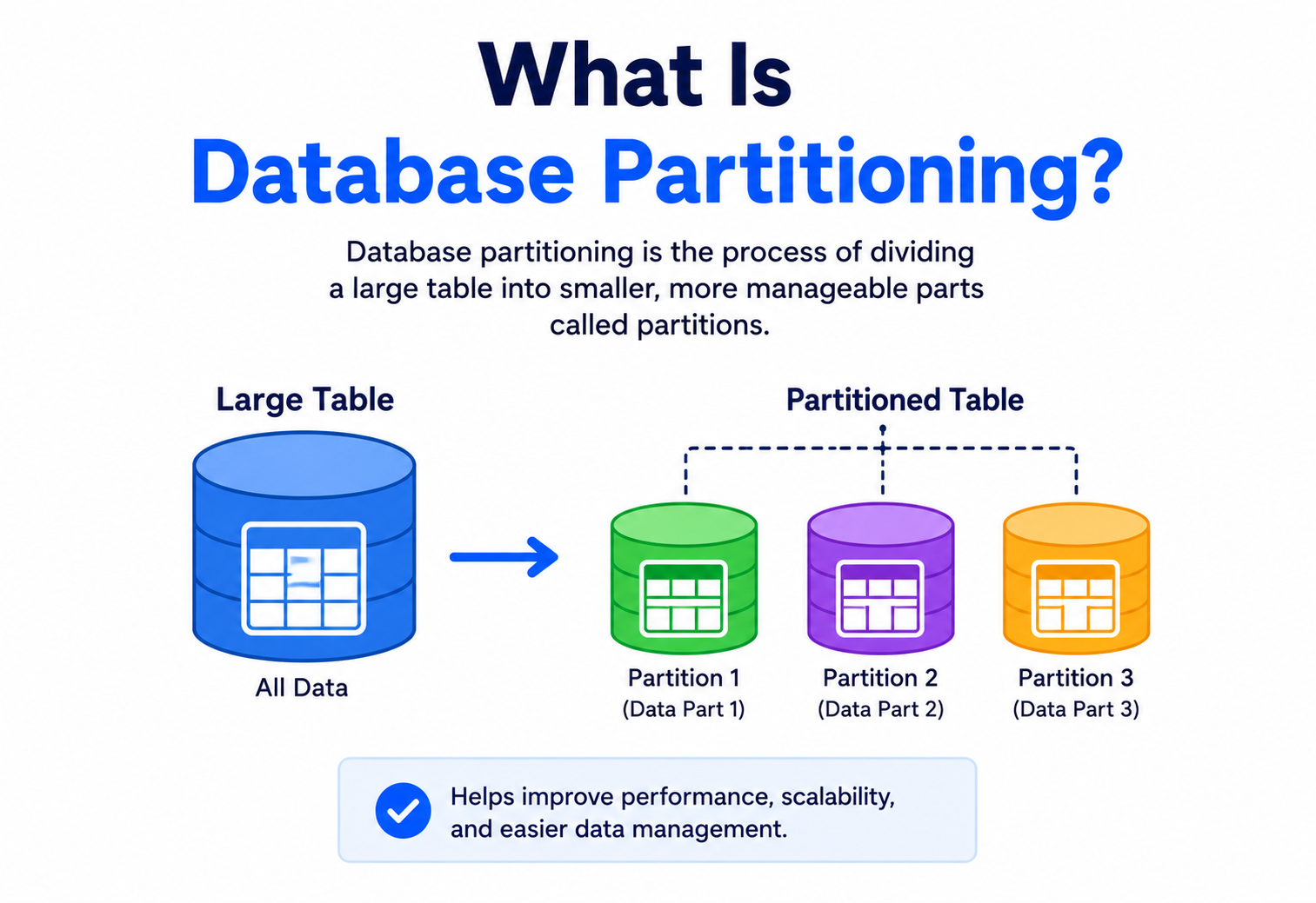
That is, almost exactly, what database partitioning is. As an application grows and its data grows with it, storing everything in a single table on a single machine eventually stops working — queries slow down, storage runs out, and one overloaded server becomes a single point of failure. Partitioning is the technique of splitting a large table (or an entire database) into smaller, more manageable pieces called partitions, so that each piece can be stored, searched, and scaled independently.
Think of a huge city’s mail system. Instead of one giant warehouse sorting every letter in the country, mail is split by postal code into regional sorting centers. Each center only ever has to deal with mail for its own area. That’s partitioning: instead of one giant, overloaded warehouse, you get many smaller, faster, specialized ones.
Partitioning answers one question: “This table has become too big and too busy for one machine — how do we split it up so each piece stays small, fast, and manageable?”
It’s worth being clear about what partitioning is not. It is not about making a single query run faster through cleverer indexing — that’s a separate topic. It is not about copying data for safety — that’s replication, which we’ll cover later. Partitioning is purely and simply about division of labor: taking one overworked piece of storage and turning it into several pieces, each doing a smaller, more manageable job. Once you internalize that one idea, almost everything else in this guide — hash functions, routers, rebalancing, hotspots — is just the practical detail of making that division work smoothly and reliably at scale.
You don’t need to work at a company the size of Instagram or Amazon to eventually run into this problem. Even a mid‑sized application — a food delivery app with a few hundred thousand users, or a project‑management tool used by a few thousand companies — can hit a wall where one table’s write traffic alone saturates a single server’s disk. Understanding partitioning early means you’ll recognize the warning signs long before they turn into a 3 a.m. outage: dashboards showing steadily climbing disk usage, query latency that quietly creeps upward week over week, and backups that take a little longer to finish every single month, until one day they no longer finish at all inside their maintenance window.
A Short History of Splitting Data
Splitting large amounts of information into smaller chunks is not a new idea — it’s older than computers. Libraries have used the Dewey Decimal System to split books by subject since the 1870s. Postal services have split mail by region for centuries. Computing simply borrowed this idea and applied it to data.
1970s–1980s: Early Mainframes
Early relational databases ran on single, extremely expensive mainframes. When data outgrew one machine’s disks, administrators manually split files across multiple disk drives — a primitive, manual form of partitioning.
1990s: Table Partitioning Arrives
Commercial databases like Oracle (Oracle 8, 1997) introduced native “table partitioning” — letting one logical table be physically split into pieces by date range or key, transparently to the application.
2000s: The Web Scale Problem
Companies like Google, Amazon, and eBay hit a wall: no single machine, however powerful, could hold the world’s search index or every product on Earth. This forced the invention of sharding — spreading partitions across many independent machines, not just many disks on one machine.
2006–2012: NoSQL & Built‑in Sharding
Systems like Amazon Dynamo (2007), Cassandra (2008), and MongoDB (2009) were designed from day one to automatically partition and distribute data across clusters of ordinary, inexpensive machines.
2012–Today: Cloud‑Native Partitioning
Modern managed databases — Amazon DynamoDB, Google Spanner, Azure Cosmos DB, CockroachDB, Vitess (used by YouTube and Slack) — treat partitioning as an invisible, automatic background process, not something engineers manage by hand anymore.
The Problem & Motivation
To really understand why partitioning exists, picture a single, ordinary database server. It has a fixed amount of memory (RAM), a fixed amount of disk space, and a fixed number of CPU cores. That’s called vertical scaling — you can make the machine bigger by adding more RAM or a faster disk, but only up to a point. Eventually you hit the biggest, most expensive machine money can buy, and it’s still not enough.
Three separate pressures push a growing system toward this wall:
Too much data
A table with billions of rows may simply not fit on one disk, or becomes too expensive to back up and restore as a single unit.
Too many requests
Even if data fits, one machine can only answer so many reads and writes per second before it becomes the bottleneck for the entire application.
Searches get slower
Searching a 10‑million‑row index takes longer than searching a 10,000‑row index, even with the best indexing — more rows simply means more work.
Partitioning attacks all three problems at once by dividing one huge, slow, overloaded table into many smaller, fast, independently‑manageable pieces. Each piece stores less data, handles fewer requests, and can even live on its own physical machine — meaning the system as a whole can keep growing almost without limit, simply by adding more machines.
One cashier at a supermarket can serve a line of shoppers reasonably fast — until the store gets busy and the line stretches out the door. The fix isn’t to make that one cashier work faster forever; it’s to open more checkout lanes, each handling a slice of the customers. Partitioning opens more “checkout lanes” for your data.
Core Concepts & Terminology
Before going further, let’s define the words you’ll see over and over in this guide. Each one is simple once explained plainly.
One slice of the whole
What it is: One smaller slice of a larger table or dataset. Why it exists: So no single piece is too big to manage. Where it’s used: In every partitioned database, from PostgreSQL to DynamoDB. Analogy: One drawer out of a big filing cabinet. Example: A “Users” table with 100 million rows split into 10 partitions of 10 million rows each.
The routing address
What it is: The specific column (or combination of columns) used to decide which partition a row belongs to. Why it exists: Something has to determine, consistently, where each piece of data lives. Where it’s used: Chosen when the table is designed — e.g. user_id, country, or order_date. Analogy: The postal code on an envelope that tells the mail system which sorting center to send it to. Example: Partitioning an “Orders” table by customer_id so all of one customer’s orders always land in the same partition.
Partitions across servers
What it is: A specific style of horizontal partitioning where the partitions (called “shards”) live on physically separate database servers, not just separate files on one server. Why it exists: A single server has hard limits on CPU, RAM, and disk — sharding spreads the load across many servers. Where it’s used: Large‑scale systems like Instagram, Discord, and Uber. Analogy: Instead of one giant supermarket, opening ten smaller supermarkets across a city. Example: A social network splits users across 64 database servers by user_id % 64.
These words are often used interchangeably, and that’s fine in casual conversation. Technically, partitioning is the general idea of splitting data into pieces (which can all still live on one server), while sharding specifically means spreading those pieces across multiple servers. Every shard is a partition, but not every partition is a shard.
Moving data after the fact
What it is: The process of moving data between partitions after they were first created, usually because one partition grew too large or too busy compared to the others. Why it exists: Data rarely grows evenly — some partitions become “hot” while others stay quiet. Where it’s used: Automatically in systems like Cassandra and DynamoDB, or manually in older systems. Analogy: A teacher reshuffling students between classrooms because one classroom got too crowded. Example: Moving half of a busy shard’s rows onto a brand‑new, empty shard.
The overloaded slice
What it is: A partition that receives a disproportionate share of traffic or data compared to the others. Why it exists: A poorly chosen partition key can cause certain values (like a celebrity’s user ID, or “today’s date”) to attract far more activity than others. Where it’s used: A well‑known failure mode discussed constantly in system design discussions. Analogy: One checkout lane at the supermarket that everyone lines up for while the others sit empty. Example: Partitioning by country where 40% of all users happen to be in one country, overloading that single partition.
Ask every shard, merge the answers
What it is: A query that has to be sent to every single partition — because it doesn’t include the partition key — with the results then merged together before being returned. Why it exists: The router has no way to know which single partition holds the answer, so it has to ask all of them. Where it’s used: Any partitioned system, whenever a query filters or searches by a field other than the partition key. Analogy: Asking every regional mail sorting center in the country “do you happen to have a letter addressed to Jane?” because you don’t know her postal code. Example: Searching an orders table (sharded by customer_id) for a specific order_id without knowing which customer placed it.
Keep related data together
What it is: Deliberately designing the partition key so that pieces of data which are frequently used or updated together end up on the same physical partition. Why it exists: It avoids the need for expensive cross‑partition joins or transactions. Where it’s used: Systems where a “parent” record and its “child” records are almost always accessed together, like a customer and their orders. Analogy: Keeping a recipe and its list of ingredients on the same page of a cookbook, instead of scattering ingredients across an appendix. Example: Partitioning both a customers table and an orders table by the same customer_id, so a customer’s orders are always on the same shard as the customer record itself.
Types of Partitioning
There isn’t just one way to split a table. Different strategies suit different kinds of data and different kinds of queries. Here are the ones you need to know.
Horizontal Partitioning (Row‑Based)
The table is split by rows — some rows go into partition A, others into partition B, but every partition keeps all the same columns. This is the most common meaning of “partitioning” in modern systems, and is the basis of sharding.
Vertical Partitioning (Column‑Based)
The table is split by columns instead of rows. Frequently‑used columns (like a user’s name and email) live in one partition, while rarely‑used or heavy columns (like a user’s full biography or profile picture blob) live in another. Every partition has all the rows, but only some of the columns.
Horizontal partitioning is like splitting a class of 100 students into five classrooms of 20 — every classroom still teaches the full subject (math, science, art). Vertical partitioning is like splitting the school day itself — math happens in one room, art happens in another — while all 100 students pass through both.
Range Partitioning
Rows are assigned to a partition based on which range their partition key value falls into — for example, orders from January go in one partition, February in another. Simple to reason about, and great for time‑series data, but risky if activity isn’t spread evenly across the ranges (all of “today’s” traffic hits one partition).
Hash Partitioning
The partition key is run through a hash function — a formula that turns any input into a scattered, unpredictable‑looking number — and the result decides the partition. This spreads data very evenly, avoiding hotspots, but makes range queries (like “give me all orders from March”) expensive, since March’s data is now scattered across every partition.
List Partitioning
Rows are assigned to a partition based on a fixed list of matching values — for example, all customers with country = 'India' go to one partition, country = 'USA' to another. Useful when data naturally clusters into known categories.
Composite (Hybrid) Partitioning
Two strategies are combined — most commonly, data is first range‑partitioned (say, by year), and each yearly range is then hash‑partitioned again internally. This captures the benefits of both: easy time‑based cleanup, and even distribution within each time range.
| Strategy | Best For | Main Risk |
|---|---|---|
| Range | Time‑series data, ordered data | Hotspots on the most recent range |
| Hash | Even load distribution | Range queries become slow |
| List | Naturally categorical data (country, region) | Uneven category sizes |
| Composite | Large‑scale systems needing both | Added design and operational complexity |
How do you actually choose between these in practice? Start by writing down your application’s three or four most common, most performance‑sensitive queries. If most of them filter by a single, evenly‑distributed value (like a user ID), hash partitioning is usually the safe default. If your data naturally arrives in time order and you regularly query or delete by date range — like logs, events, or financial transactions — range partitioning lets you cleanly drop or archive entire old partitions without touching the rest of the table. If your data already falls into a small number of well‑known categories, list partitioning keeps things intuitive. And if you find yourself needing the strengths of two of these at once, composite partitioning — despite its added complexity — is usually a better long‑term choice than trying to force one single strategy to do a job it wasn’t designed for.
Architecture & Components
A partitioned database isn’t just “many small databases sitting side by side” — it needs extra machinery to work correctly. Here are the pieces that show up in almost every partitioned system.
Partition / Shard
The actual physical slice of data — a table, file, or entire server holding one portion of the dataset.
Partition Key
The column(s) used to decide, for any given row, which partition it belongs to.
Router / Query Coordinator
The layer that looks at an incoming query, figures out which partition(s) it needs, and forwards the request there.
Metadata / Config Store
A small, highly‑available store that tracks which partition key ranges live on which physical shard right now.
The router is the piece most people forget about when first learning partitioning, but it’s arguably the most important. Without it, every application would need to hard‑code knowledge of exactly which server holds which data — and that knowledge would break the moment a shard is added, removed, or rebalanced. The router keeps that complexity hidden behind a single, stable interface.
The metadata store itself becomes a critical dependency — if it goes down or serves stale information, queries can be routed to the wrong shard entirely. Production systems replicate this metadata store heavily and cache it aggressively on the client side.
There’s one more architectural choice worth understanding: where does the router actually live? There are two common answers. In a “proxy‑based” design, the router is a separate piece of infrastructure that every application server talks to — like Vitess’s VTGate component sitting in front of sharded MySQL. In a “smart client” design, the routing logic is built directly into a library that application code imports — the application itself computes the hash and talks straight to the right shard, skipping the extra network hop of a separate proxy. Proxy‑based routing is simpler to operate and upgrade centrally; smart‑client routing is faster because it removes a hop, at the cost of every application needing to stay in sync with routing logic changes.
How Routing Works Internally
Let’s trace exactly what happens, step by step, when a query like SELECT * FROM orders WHERE customer_id = 4521 is sent to a partitioned database that shards by customer_id using hash partitioning across 4 shards.
Extract the Partition Key
The router inspects the query and pulls out the value of the partition key — here, customer_id = 4521.
Apply the Hash Function
The router computes hash(4521) % 4, which deterministically produces the same result every single time this value is hashed.
Look Up the Shard Map
The result (say, 2) is looked up against the current shard map to find which physical server currently owns “bucket 2.”
Forward the Query
The query is sent only to that one shard — not to all four — because the router already knows exactly where the answer lives.
Return the Result
The shard executes the query locally and returns the rows, which the router passes straight back to the application.
Notice that steps 1–3 all happened before any actual database work occurred. This is the key insight: a good partitioning scheme lets the system know exactly where to look before touching disk, instead of searching every shard and combining the results (which is far slower, and called a “scatter‑gather” query).
Data Flow & Lifecycle
Beyond a single read, it helps to see the full lifecycle of data in a partitioned system — from the moment it’s written, to the moment a partition needs to be split.
The Write Path
When a new row is inserted, the same routing logic runs in reverse: the partition key is extracted from the new row, hashed or matched against a range, and the row is written directly to the owning shard. In systems that also replicate data for safety, the write is first sent to the shard’s primary copy, then copied to one or more replica copies before the write is confirmed as successful.
The Read Path
Reads follow the same routing as writes when the query includes the partition key. When a query does not include the partition key (for example, searching by email instead of customer_id), the router often has no choice but to send the query to every shard and merge the results — a slower “scatter‑gather” pattern, which is one of the most important trade‑offs to understand about partitioning.
Growth & Splitting
As a partition accumulates more data or traffic, most modern systems automatically detect it crossing a size or load threshold, and split it into two smaller partitions — copying roughly half the data to a new shard, updating the metadata store, and only then deleting the now‑duplicated original rows.
This copying step deserves a closer look, because it’s where most of the real engineering difficulty lives. While the split is happening, the original partition is still receiving live reads and writes from real users — the system can’t simply pause traffic for the minutes or hours a large copy might take. The standard solution is to copy the bulk of the data first as a background “snapshot,” and then replay every write that happened during the copy (tracked in a change log) onto the new shard before finally flipping the metadata store to point traffic at it. Only once the new shard is fully caught up does the system consider the split complete and safe to clean up the duplicated rows on the original shard.
Splitting a live shard without downtime is one of the hardest engineering problems in distributed databases — systems like MongoDB and Cassandra spend enormous engineering effort making sure reads and writes keep working correctly while data is being copied in the background.
Partitioning Strategies in Code
Reading about hashing and ranges is one thing — seeing the actual logic makes it click. Below are small, self‑contained Java examples showing how a router might decide which shard owns a given key. In production, these ideas are usually implemented inside the database engine itself, but writing them by hand is the fastest way to truly understand them.
Simple Hash Partitioning
public class HashPartitioner {

    private final int numShards;

    public HashPartitioner(int numShards) {
        this.numShards = numShards;
    }

    // Decide which shard a given key belongs to
    public int getShard(String partitionKey) {
        int hash = Math.abs(partitionKey.hashCode());
        return hash % numShards;
    }

    public static void main(String[] args) {
        HashPartitioner partitioner = new HashPartitioner(4);
        System.out.println("customer_4521 -> shard " + partitioner.getShard("4521"));
        System.out.println("customer_9981 -> shard " + partitioner.getShard("9981"));
    }
}
This works well for even distribution, but it has a serious weakness: if you ever change numShards (say, from 4 to 5, because you added a machine), the modulo result changes for almost every single key — meaning almost all data would need to be reshuffled at once. That’s exactly the problem consistent hashing was invented to solve.
Consistent Hashing
Instead of mapping keys directly to shard numbers, consistent hashing places both shards and keys onto a conceptual circle (a “hash ring”). A key belongs to the first shard found walking clockwise around the ring. Adding or removing a shard only affects the small slice of the ring next to it — not the entire dataset.
import java.util.SortedMap;
import java.util.TreeMap;

public class ConsistentHashRing {

    private final SortedMap<Integer, String> ring = new TreeMap<>();
    private final int virtualNodes;

    public ConsistentHashRing(int virtualNodes) {
        this.virtualNodes = virtualNodes;
    }

    public void addShard(String shardName) {
        for (int i = 0; i < virtualNodes; i++) {
            int position = (shardName + "#" + i).hashCode();
            ring.put(position, shardName);
        }
    }

    public void removeShard(String shardName) {
        ring.values().removeIf(v -> v.equals(shardName));
    }

    public String getShard(String key) {
        int hash = key.hashCode();
        SortedMap<Integer, String> tail = ring.tailMap(hash);
        int position = tail.isEmpty() ? ring.firstKey() : tail.firstKey();
        return ring.get(position);
    }
}
The virtualNodes trick matters in practice: giving each real shard many points on the ring (instead of just one) keeps the data spread evenly, even when there are only a handful of physical shards.
Range Partitioning
import java.time.LocalDate;
import java.util.NavigableMap;
import java.util.TreeMap;

public class RangePartitioner {

    // Maps the START date of a range to the shard that owns it
    private final NavigableMap<LocalDate, String> ranges = new TreeMap<>();

    public void addRange(LocalDate startDate, String shardName) {
        ranges.put(startDate, shardName);
    }

    public String getShard(LocalDate orderDate) {
        return ranges.floorEntry(orderDate).getValue();
    }

    public static void main(String[] args) {
        RangePartitioner partitioner = new RangePartitioner();
        partitioner.addRange(LocalDate.of(2024, 1, 1), "shard-2024");
        partitioner.addRange(LocalDate.of(2025, 1, 1), "shard-2025");
        partitioner.addRange(LocalDate.of(2026, 1, 1), "shard-2026");

        System.out.println(partitioner.getShard(LocalDate.of(2025, 6, 15))); // shard-2025
    }
}Notice the pattern in all three examples: every strategy answers the exact same question — “given this key, which shard owns it?” — they just use different math to answer it. That single function is the heart of every partitioning system.
Advantages, Disadvantages & Trade‑offs
Partitioning is powerful, but it is never free. Every benefit below comes paired with a genuine cost, and a good engineer weighs both before reaching for it.
Advantages
- Enables near‑limitless horizontal scaling by adding more machines
- Smaller partitions mean faster queries, backups, and index rebuilds
- A failure in one partition doesn’t necessarily take down the whole system
- Different partitions can be tuned or placed closer to their users geographically
Disadvantages
- Queries that don’t include the partition key become slow “scatter‑gather” operations
- Joins across partitions are difficult, slow, or simply not supported
- Maintaining uniqueness (like auto‑incrementing IDs) across partitions gets tricky
- Rebalancing and operating a partitioned cluster adds real operational complexity
Partitioning trades simplicity for scale — and it should only be adopted once simplicity has genuinely run out of room.
The Auto‑Increment ID Problem
Here’s a trade‑off many newcomers don’t see coming. In a single, unpartitioned database, an auto‑incrementing primary key (1, 2, 3, 4…) is trivial — the database just remembers the last number it used. Once a table is split across multiple shards, that trick breaks: if shard A and shard B both independently count “1, 2, 3…”, you’ll end up with duplicate IDs across the whole system. Common fixes include reserving separate ID ranges per shard (shard A uses 1,000,000–1,999,999, shard B uses 2,000,000–2,999,999), using globally unique identifiers like UUIDs instead of sequential numbers, or using a dedicated, centralized ID‑generation service (a pattern popularized by Twitter’s “Snowflake” ID generator, which packs a timestamp, a shard number, and a counter into a single 64‑bit number).
Performance & Scalability
The entire point of partitioning is performance under growth, so it’s worth being precise about what actually gets faster, and why.
A query that must scan an entire table on a single 10‑million‑row database might take several seconds. Split evenly across 10 shards, that same query — if it can be routed to a single shard — now scans roughly 1 million rows, often finishing in a fraction of the time. Even scatter‑gather queries benefit somewhat, because the 10 shards can be searched in parallel rather than one after another.
Scalability isn’t only about a single query, though — it’s about how much total traffic the whole system can handle. A single database server might comfortably support 5,000 writes per second. Ten independent shards, each handling their own slice of the write traffic, can support closer to 50,000 writes per second in aggregate — because they’re not competing for the same CPU, memory, or disk.
This scaling is not automatic or infinite. It only holds if data and traffic are spread evenly across partitions. A single hotspot can single‑handedly erase all the performance gains of partitioning the other 99% of the data correctly.
There’s also a subtler performance cost worth understanding: coordination overhead. The moment a query needs to touch more than one shard — a scatter‑gather query, or a transaction spanning two partitions — the system has to wait for the slowest of those shards to respond, and often needs extra network round‑trips to keep the results consistent. This means a poorly‑chosen partition key doesn’t just cause a hotspot; it can make previously‑simple operations measurably slower than they were on a single, unpartitioned database, even though the total system is handling far more overall traffic. This is exactly why so much of this guide keeps returning to the same point: the partition key has to match real query patterns, not just split data evenly for its own sake.
A useful mental model: think of total system throughput as roughly (throughput per shard) × (number of shards) × (efficiency factor), where the efficiency factor drops below 1.0 the more cross‑shard coordination a workload requires. A well‑partitioned system with efficient, single‑shard queries can push that factor close to 1.0 — near‑linear scaling. A poorly‑partitioned system full of scatter‑gather queries might see an efficiency factor closer to 0.3 or lower, meaning adding shards yields rapidly diminishing returns.
High Availability & Reliability
Partitioning and replication solve two different problems, and it’s important not to confuse them: partitioning spreads data out to handle scale, while replication copies data to handle failure. Production systems almost always use both together — each partition is itself replicated across multiple machines, so losing one server doesn’t mean losing that slice of data.
The CAP Theorem, in Plain Words
When a network problem splits a cluster into two groups that can’t talk to each other (a “partition” in the networking sense — a different meaning of the word than data partitioning, unfortunately), a distributed database must choose between:
- Consistency — every read gets the most recent write, even if it means refusing some requests during the split.
- Availability — every request gets some answer, even if it might be slightly out of date.
You cannot have perfect versions of both at the same time during a network split — this is the famous CAP theorem. Systems like traditional relational databases with strong consistency lean toward the “C” side; systems like Cassandra and DynamoDB, by default, lean toward the “A” side, favoring uptime over perfect freshness.
Most real applications don’t need to consciously “pick” CAP — most managed cloud databases make sensible defaults, and let you tune consistency per‑query when it truly matters (like a bank balance) versus when it doesn’t (like a “likes” counter).
What Happens When a Shard’s Primary Fails
Availability in a partitioned system isn’t all‑or‑nothing — it’s per‑shard. If Shard 3’s primary server crashes, only the data living on Shard 3 is affected; Shards 1, 2, and 4 keep serving reads and writes completely normally. Most replicated systems run an automatic failover process: the remaining replicas of Shard 3 detect the primary is unreachable (usually through a heartbeat mechanism), elect one of themselves as the new primary through a consensus protocol like Raft or Paxos, and update the metadata store so the router starts sending Shard 3’s traffic to the new primary — often within a few seconds. This is one of partitioning’s quieter benefits: a total outage becomes a partial, contained one, affecting only the slice of users whose data happened to live on the failed shard.
Security Considerations
Splitting data across many machines multiplies the number of places that need to be secured — a partitioned system has a larger “surface area” than a single database, and that has real consequences.
Encrypt every shard
Data must be encrypted at rest and in transit on every single shard, not just the ones an engineer remembers to configure.
Consistent permissions
A user’s permissions must be enforced identically no matter which shard actually answers their query.
Where data physically lives
Laws like GDPR often require certain users’ data to stay within a specific country — a use case partitioning is uniquely well‑suited to solve, by routing EU users to EU‑based shards.
Unified logging
Security logs from every shard need to be centralized, or an attacker could exploit gaps between separately‑monitored machines.
Interestingly, partitioning by geography is now a common way to satisfy privacy laws rather than complicate them — a system that already routes European users’ data to European shards has a natural answer to “does this data ever leave the EU?”
There’s also a genuine security upside worth mentioning: blast radius reduction. If an attacker manages to compromise credentials for one shard, or exploits a vulnerability specific to one server, the damage is naturally contained to whatever slice of data lives on that shard — not the entire dataset. This is the same principle behind splitting a ship into watertight compartments: a hole in one compartment doesn’t necessarily sink the whole vessel. That said, this benefit only holds if each shard genuinely uses separate credentials and separate network access controls — if every shard shares one master database password, the “watertight compartments” become purely theoretical.
Monitoring, Logging & Metrics
You cannot fix a hotspot you cannot see. Operating a partitioned system well depends heavily on watching the right numbers, per shard, all the time.
| Metric | Why It Matters |
|---|---|
| Rows / storage size per shard | Reveals uneven data growth before it becomes a crisis |
| Queries per second, per shard | Catches hotspots caused by traffic, not just data size |
| P99 query latency, per shard | A single slow shard can silently drag down overall app performance |
| Replication lag | Shows how far behind replicas are from the primary, per shard |
| Scatter‑gather query count | High counts often reveal a partition key that doesn’t match real query patterns |
Most teams build a dashboard that shows these numbers side‑by‑side across every shard, specifically so that an unusually tall bar (a hotspot) jumps out visually. Alerts are typically set not on absolute values, but on relative imbalance — for example, “alert if any shard has more than 3x the average load of the others.”
Logging deserves special mention in a partitioned system, because a single user request can touch multiple shards (a router, one or more shards, and possibly a metadata store), and debugging a slow or failed request means piecing together logs from all of them. The standard fix is a correlation ID — a unique identifier generated when a request first enters the system, then passed along and logged at every single hop it makes. Searching for that one ID in a centralized logging system (like the ELK stack or Datadog) reconstructs the full journey of a request across every shard it touched, turning what would otherwise be a scavenger hunt through dozens of separate log files into a single, readable timeline.
Deployment & Cloud
Very few teams build partitioning logic entirely from scratch today. Modern cloud databases bake it in, and the job becomes choosing the right partition key rather than writing the routing engine yourself.
DynamoDB
Fully‑managed; you choose a “partition key” at table creation, and AWS handles all sharding, splitting, and rebalancing automatically.
Spanner
Globally distributed relational database that automatically splits data into ranges and moves them across regions for both scale and latency.
Cosmos DB
Requires choosing a “partition key” much like DynamoDB, with automatic, transparent scaling behind the scenes.
Vitess & Citus
Add automatic sharding on top of ordinary MySQL (Vitess, used by YouTube) or PostgreSQL (Citus), for teams that want to keep their existing SQL database.
Even relational databases that weren’t originally built for sharding — like PostgreSQL and MySQL — support native table partitioning (splitting one big table into range‑ or list‑based partitions on a single server) as a stepping stone before a team needs true multi‑server sharding.
“Table partitioning” (one server, multiple physical pieces of one logical table) and “sharding” (many servers) solve related but different‑sized problems. Most teams should exhaust the first before reaching for the second — it’s far simpler to operate.
Cost is a practical, if less glamorous, part of this decision too. A managed, auto‑sharding database like DynamoDB or Cosmos DB removes almost all operational burden, but usually charges based on provisioned or consumed throughput per partition — meaning a poorly distributed partition key doesn’t just cause a performance problem, it can directly inflate the monthly bill, since hot partitions may require over‑provisioning capacity for the whole table just to keep one busy slice from throttling. Self‑managed sharding (running your own Vitess or Citus cluster) trades that convenience for lower per‑unit infrastructure cost, at the price of needing engineers who understand how to operate it.
Partitioning, Caching & Load Balancing
Partitioning rarely works alone — it typically sits alongside two close relatives, and it’s easy to mix them up when first learning system design.
| Technique | What It Splits | Solves |
|---|---|---|
| Partitioning | The data itself, at rest | Too much data / too much load for one storage server |
| Load Balancing | Incoming requests, before they reach any server | Too many requests for one application server to handle |
| Caching | Nothing — it stores a temporary copy of hot data close to where it’s needed | Repeated, expensive reads of the same data |
In a typical large‑scale architecture, a load balancer spreads incoming user requests across many identical application servers; those servers check a cache (like Redis) first for frequently‑requested data; and only on a cache miss do they fall through to the partitioned database, where the router sends the query to the correct shard. All three techniques attack the same underlying problem — too much of something for one machine — from different angles.
APIs & Microservices
Partitioning shows up at the architecture level too, not just inside a single database. In a microservices architecture, it’s common practice for each service to own its own database — which is itself a form of functional partitioning: instead of splitting one table by row, the entire dataset is split by business function (a “Users” database, an “Orders” database, a “Payments” database).
This nests neatly: a system can be functionally partitioned by service, and then each individual service’s database can itself be horizontally partitioned by row, if that one service grows large enough on its own. Instagram’s user data, for instance, is both functionally separated from its media‑serving systems, and internally sharded by user ID within its own datastore.
APIs also need to be designed with partitioning in mind. A well‑designed API for a partitioned system typically requires the partition key as part of the request — for example, requiring both a customerId and an orderId to fetch a specific order, rather than the orderId alone — because that small design choice is what lets the API gateway or service route the request directly to the correct shard, instead of falling back on an expensive scatter‑gather lookup across every shard just to find one order.
Design Patterns & Anti‑patterns
Some strategies show up again and again in production systems because they work at scale. Others keep breaking systems for the same reasons over and over — recognizing them by name is half the battle.
Pattern: Directory‑Based Partitioning
Instead of computing a shard with math (hash or range), a lookup table explicitly maps each key to its shard. This is the most flexible strategy — rebalancing is just updating a row in the lookup table — but that lookup table itself must be fast and highly available, since every single query depends on it. Because the mapping is explicit rather than computed, this pattern also makes it easy to move a single “hot” customer’s data onto its own dedicated shard, without disturbing the hashing or ranges used for everyone else — a technique sometimes called “shard isolation,” commonly used for the largest, highest‑traffic tenants in multi‑tenant SaaS systems.
Pattern: Consistent Hashing with Virtual Nodes
As shown earlier in code, giving every physical shard many positions on the hash ring keeps load evenly spread even with few shards, and minimizes data movement when shards are added or removed. This is the industry‑standard approach used by Cassandra, DynamoDB, and many CDNs.
Anti‑pattern: Partitioning by a Low‑Cardinality Key
Choosing a partition key with very few possible values — like status (only “active” or “inactive”) or boolean_flag — guarantees a hotspot, because all the data funnels into just a handful of buckets no matter how many shards exist.
Anti‑pattern: Ignoring Query Patterns
Picking a partition key based on what feels “natural” (like an auto‑incrementing primary key) without checking how the application actually queries the data almost always leads to expensive scatter‑gather queries in production. The partition key should match the most common, most performance‑critical query — not necessarily the most “obvious” column.
Anti‑pattern: Cross‑Shard Transactions as a Habit
Needing a transaction that updates rows across two different shards is sometimes unavoidable, but relying on it constantly is a sign the partitioning boundary was drawn in the wrong place — related data that’s frequently updated together should usually live in the same partition.
Re‑sharding an already‑live, already‑large production system is one of the most difficult and risky operations in all of database engineering. Choosing a good partition key on day one is far cheaper than fixing a bad one later.
Best Practices & Common Mistakes
Most of what separates a partitioned system that scales gracefully for years from one that requires a painful, high‑risk re‑sharding project six months after launch comes down to a handful of decisions made early, before a single line of application code depends on them. The list below distills the lessons from the patterns, anti‑patterns, and real‑world examples covered throughout this guide into a single, practical checklist.
Best practices
- Choose a partition key that matches your most frequent, highest‑traffic query
- Favor high‑cardinality keys (many possible values) to spread load evenly
- Keep frequently‑joined or frequently‑updated‑together data in the same partition
- Monitor per‑shard metrics continuously, not just aggregate system‑wide metrics
- Start with native single‑server table partitioning before jumping to multi‑server sharding
Common mistakes
- Choosing an auto‑increment ID as the partition key without checking query patterns
- Partitioning by a field with very few possible values (creating instant hotspots)
- Designing the schema before ever measuring real, expected query traffic
- Forgetting that cross‑shard joins and transactions are slow, and relying on them anyway
- Treating rebalancing as an afterthought instead of planning for it from day one
Real‑World & Industry Examples
The same underlying idea — split the data, route the queries, keep the pieces even — shows up in wildly different systems, tuned to each company’s workload.
Sharded PostgreSQL
Instagram famously shards its Postgres databases by user ID, using logical shards mapped onto a smaller number of physical database servers — letting them add hardware without reshuffling application logic.
Cassandra, then ScyllaDB
Discord partitions chat messages by channel ID, so an extremely busy server’s messages don’t overwhelm the partition holding a quiet one — they later migrated to ScyllaDB for even better per‑shard performance.
DynamoDB
Built from the internal “Dynamo” paper (2007) specifically to solve Amazon’s shopping‑cart availability problems at massive scale, using consistent hashing across partitions from the ground up.
Schemaless / MySQL sharding
Uber built a custom sharding layer atop MySQL to handle trip data partitioned geographically and by time, matching how their queries actually access recent, regional trip data.
Vitess
YouTube outgrew a single MySQL server for its metadata and built Vitess — later open‑sourced and now used by Slack and Square — to shard MySQL transparently while keeping full SQL compatibility for application engineers.
Range & hash sharding
MongoDB offers both range‑based and hash‑based sharding out of the box, letting teams pick a “shard key” and delegate all splitting and balancing to the database itself as collections grow.
Notice a pattern across every one of these companies: none of them started with a heavily‑sharded architecture. All of them began with a single, ordinary database, and only introduced partitioning once real, measured growth demanded it — reinforcing one of the most important lessons in this entire guide. In several of these cases (Instagram, Uber, YouTube), the sharding layer was built as a thin, custom‑engineered piece of infrastructure specifically because, at the time, no off‑the‑shelf tool did exactly what they needed — a strong signal that partitioning decisions tend to be deeply tied to a company’s specific query patterns, not a one‑size‑fits‑all recipe copied from a textbook.
Frequently Asked Questions
The questions that come up almost every time an engineer starts learning or teaching partitioning — answered briefly, without hand‑waving.
Is partitioning the same as sharding?
Nearly, but not exactly. Partitioning is the general idea of splitting data into smaller pieces; sharding specifically means those pieces live on separate physical servers. Every shard is a partition, but a partition doesn’t have to be a shard.
Do small applications need partitioning?
Almost never at first. A single well‑tuned database server can comfortably handle millions of rows and thousands of requests per second. Partitioning adds real operational complexity, so it should be introduced only once genuine, measured growth requires it.
What happens if I choose the wrong partition key?
You’ll likely see uneven “hot” partitions, slow scatter‑gather queries for common operations, and eventually need to re‑shard the entire dataset — a difficult, risky, and time‑consuming migration on a live system.
Can I change my partition key later?
Yes, but it typically requires re‑sharding — copying and re‑routing the entire dataset according to the new key — which is one of the most operationally risky projects a database team can undertake, so it’s worth investing real time in choosing well up front.
Does partitioning replace the need for replication?
No — they solve different problems. Partitioning spreads data out for scale; replication copies data for durability and availability. Production systems use both together, typically replicating each individual partition.
Is partitioning only for NoSQL databases?
No. Relational databases like PostgreSQL, MySQL, and Oracle all support native table partitioning, and can be combined with tools like Citus or Vitess to add full multi‑server sharding while keeping standard SQL.
How many partitions should I start with?
There’s no universal number — it depends on expected data volume and traffic. A common practical approach is to start with more logical partitions than you need physical servers for (for example, 128 logical shards mapped onto just 4 physical machines at launch), so that future growth only requires moving existing logical shards onto new machines, rather than re‑partitioning the data itself.
What’s the difference between partitioning and federation?
Federation (sometimes called “functional partitioning”) splits a database by subject area — a Users database, a Products database, a Reviews database — each potentially with a completely different schema. Partitioning, in the narrower sense used throughout this guide, splits a single table’s rows or columns while keeping one consistent schema across every piece.
Key Takeaways
Six sentences that, if you remember nothing else from this guide, will still make you a noticeably better engineer the next time a database starts groaning under its own weight.
Remember this
- Partitioning splits a large dataset into smaller, more manageable pieces so no single machine has to hold or serve everything.
- Horizontal partitioning splits by rows; vertical partitioning splits by columns; sharding specifically means the pieces live on separate physical servers.
- The partition key is the single most important design decision — it should match your most frequent, most important query pattern.
- Hash partitioning spreads load evenly but hurts range queries; range partitioning is intuitive but risks hotspots on recent data; consistent hashing minimizes reshuffling when shards change.
- Partitioning solves scale, replication solves durability — real systems need both, working together.
- Start simple. Every major company that shards today started with one plain database, and only partitioned once real growth demanded it.