What Is Data Warehousing?
A complete, beginner‑friendly guide to how companies like Netflix, Amazon, and Uber store years of business data and turn it into decisions — explained from first principles, with diagrams, code, and real production practices.
Introduction & History
Imagine you own a toy shop. Every day you sell toys, and every day you write down what you sold in a small notebook. After one year, you have 365 notebook pages. Now your mother asks you: “Which toy sold the best in December over the last five years?”
To answer that, you would need to dig through five years of notebooks, page by page, add up numbers by hand, and hope you don’t make a mistake. That is slow, tiring, and error‑prone.
Now imagine instead that every night, you copied the important numbers from your notebook into one big, well‑organised ledger — sorted by toy, by month, by year — so that any question about your sales history could be answered in seconds. That big, organised ledger is exactly what a data warehouse is, except it stores information for entire companies instead of a toy shop.
A data warehouse is like a giant, well‑organised library for a company’s history. A normal database is like the librarian’s daily “in‑tray” — new books (transactions) arrive constantly and get processed one at a time. A data warehouse is the permanent archive section, where books are catalogued, cross‑referenced, and arranged so you can instantly find “every mystery novel published between 1990 and 2000,” instead of checking every single book one by one.
1.1 What Is Data Warehousing?
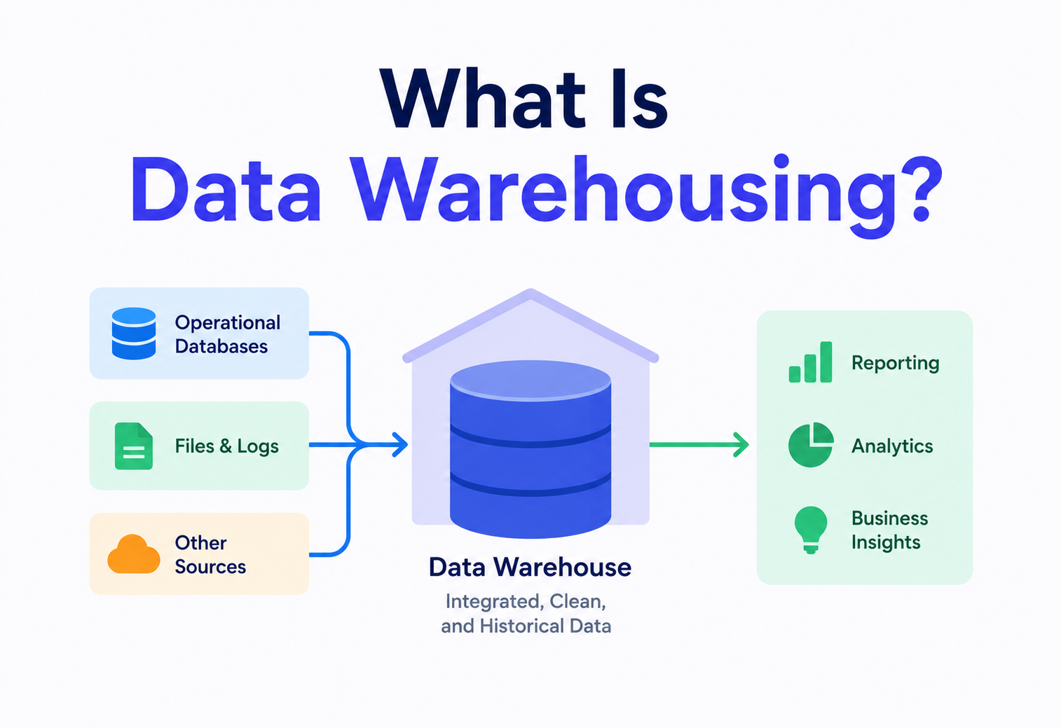
Data warehousing is the process of collecting data from many different sources inside a company (sales systems, websites, mobile apps, customer support tools, inventory systems, and more), cleaning and organising that data, and storing it in one central place called a data warehouse. This central place is specially designed to answer big analytical questions quickly, like “What were our total sales by region last quarter?” or “Which customers are most likely to stop using our app?”
A data warehouse is not just a bigger database. It is a database built with a completely different goal in mind. A normal (“operational”) database is built to record things fast — one order at a time, one login at a time. A data warehouse is built to look back across millions or billions of those records at once and find patterns, trends, and totals.
1.2 A Short History
Data warehousing did not appear overnight. It grew out of a real business pain point that got worse as computers became common in offices.
- 1970sThe age of isolated systems. Companies started using computers to track sales, payroll, and inventory — but each department had its own separate system. The sales team’s data lived in one place, finance’s data lived in another, and nobody could easily combine them.
- 1980sThe rise of decision support systems. Businesses realised that if they could combine data from all departments, they could make smarter decisions. Early “decision support systems” (DSS) were built, but they were slow, custom‑built, and expensive.
- 1988IBM coins the foundational idea. IBM researchers Barry Devlin and Paul Murphy published a paper describing a “business data warehouse” — a single place to store data for reporting, separate from the everyday operational systems.
- 1990sBill Inmon and Ralph Kimball. Two experts shaped the field with different philosophies. Bill Inmon, often called the “father of data warehousing,” pushed a top‑down approach (build one central, highly normalised warehouse first). Ralph Kimball promoted a bottom‑up approach (build small, business‑focused “data marts” using simpler star schemas, then connect them). Both approaches are still taught and used today.
- 2000sSpecialised appliances. Companies like Teradata, Netezza, and later Vertica built hardware and software specifically optimised for warehouse‑style queries, dramatically speeding up analytics on large datasets.
- 2010sThe cloud and big data era. Cloud data warehouses like Amazon Redshift, Google BigQuery, and Snowflake removed the need to buy physical hardware. At the same time, “data lakes” emerged to store huge amounts of raw, unstructured data cheaply. This led to hybrid ideas like the “data lakehouse.”
- 2020sReal‑time and AI‑ready warehouses. Modern warehouses now support near real‑time data streaming, automatic scaling, built‑in machine learning tools, and tight integration with AI systems — while still keeping the core idea from the 1980s: one trusted place for company‑wide answers.
Interviewers sometimes ask “Inmon vs. Kimball?” or “why did data warehouses evolve?” Knowing this timeline shows you understand data warehousing as a solution to a real, ongoing business problem — not just a piece of software to memorise.
Problem & Motivation
To understand why data warehouses exist, you first need to understand the systems that came before them, and why those systems struggle with big analytical questions.
2.1 The Problem: Data Is Scattered and Systems Are Busy
A modern company might have dozens of separate systems: an app database for user accounts, a payments system for transactions, a support ticket tool, a marketing email platform, and a mobile analytics tool. Each system is really good at its own specific job, but terrible at answering big‑picture questions that span all of them.
There are three core problems:
1. Data is scattered
Sales data lives in one system, customer support data in another, and website clicks in a third. There is no single place to ask “how do support tickets affect whether a customer buys again?”
2. Operational systems get slow
The database that runs your checkout page needs to respond in milliseconds. If someone runs a huge report on that same database, it can slow down real customers trying to buy something right now.
3. Data formats don’t match
One system might store a date as “2024‑05‑01” and another as “May 1, 2024.” One might call a customer a “user_id” and another a “client_number.” Without cleanup, comparing them is like comparing notes written in different languages.
Picture a hospital. The pharmacy has its own record book, the emergency room has its own, and the billing office has its own. If the hospital director wants to know “how many patients who visited the ER in the last year were later admitted, and what did that cost the hospital?”, nobody can answer that quickly by flipping through three different books kept in three different rooms, updated by three different staff, in three different formats. The hospital needs one master record, reorganised specifically for answering exactly those kinds of big questions.
2.2 OLTP vs. OLAP: The Core Distinction
This is one of the most important ideas in this entire tutorial, and it comes up constantly in interviews. Systems that record everyday transactions are called OLTP systems. Systems built for analysis are called OLAP systems.
| OLTP (Online Transaction Processing) | OLAP (Online Analytical Processing) | |
|---|---|---|
| Purpose | Record day‑to‑day operations (an order, a login, a payment) | Analyse historical data for trends and decisions |
| Example query | “Insert this new order for customer #4521” | “What was total revenue by region for each of the last 8 quarters?” |
| Data volume per query | A few rows | Millions or billions of rows |
| Speed needed | Milliseconds | Seconds to minutes is acceptable |
| Data freshness | Always current, up‑to‑the‑second | Often refreshed hourly or daily (though real‑time is growing) |
| Design goal | Avoid duplicate data (normalised) | Fast reads across huge datasets (often denormalised) |
| Typical users | Applications, end customers | Analysts, executives, data scientists, dashboards |
| Example tools | MySQL, PostgreSQL, Oracle (for apps) | Snowflake, BigQuery, Redshift, Teradata |
Beginners often think a data warehouse is “just a bigger database.” It’s more accurate to say a data warehouse is a database with a different design philosophy: it accepts slower single‑row inserts in exchange for extremely fast large‑scale reads, which is the opposite trade‑off an OLTP database makes.
2.3 Why Not Just Run Reports on the Live Database?
You might ask: “Why not just run the big report directly on the app’s database?” Three reasons:
- Performance risk — a heavy analytical query can lock tables or consume resources, slowing down or even crashing the live application that real customers are using.
- Limited history — operational databases are often trimmed or archived to stay fast, so old data may not even exist there anymore.
- No unified view — the operational database only knows about its own slice of the business (e.g. orders), not marketing, support, or finance data.
This is the core motivation for data warehousing: separate the system that records the business from the system that explains the business.
Core Concepts
Before going into architecture, let’s build a solid vocabulary. Every term below is something you will see again and again in real jobs and interviews.
WhatA central repository of integrated data from one or more different sources, structured specifically for query and analysis rather than transaction processing.
WhyTo give a company one trustworthy, unified, historical view of its data.
WhereBusiness intelligence dashboards, financial reporting, executive decision‑making, machine learning feature stores.
ExampleA retail company stores five years of every purchase, refund, and customer interaction in a warehouse so analysts can study buying patterns.
WhatA three‑step process to move data into a warehouse: Extract data from source systems, Transform it into a clean, consistent format, and Load it into the warehouse.
WhyRaw data from different systems is messy and inconsistent; it must be cleaned and reshaped before it’s useful for analysis.
Think of making a fruit salad. Extract is picking fruits from different trees (apple tree, orange tree, banana tree). Transform is washing, peeling, and cutting them into similar‑sized pieces. Load is putting all the prepared pieces into one big bowl, ready to serve.
WhatA more modern variant where raw data is loaded into the warehouse first, and transformation happens afterward, using the warehouse’s own powerful computing engine.
WhyModern cloud warehouses (like Snowflake or BigQuery) are so powerful that it’s often faster and simpler to dump raw data in and transform it with SQL inside the warehouse, rather than transforming it beforehand on separate servers.
ExampleA company loads raw, messy JSON logs from its app directly into BigQuery, then uses SQL (often managed by a tool called dbt) to clean and reshape that data into neat tables.
WhatThe blueprint that defines how tables, columns, and relationships are organised.
WhyWithout a plan, data would be a chaotic pile of numbers and text with no clear meaning or connections.
Star Schema
A central fact table (the “who did what” — e.g. sales transactions) surrounded by several dimension tables (descriptive details — e.g. product, customer, date, store). It looks like a star when you draw it, hence the name.
Snowflake Schema
Similar to a star schema, but the dimension tables are further broken down into sub‑tables to reduce duplicate data. It looks like a snowflake with extra branches.
Imagine a school report‑card system. The fact table is “exam scores” — one row per student, per subject, per exam. The dimension tables are “students” (name, class, age), “subjects” (name, teacher), and “exam dates.” A star schema keeps each dimension as one simple table. A snowflake schema might split “students” further into “students” and a separate “classes” table, connected together — more organised, but requires a few more steps to look something up.
3.5 Fact Table vs. Dimension Table
| Fact Table | Dimension Table | |
|---|---|---|
| Contains | Measurable events/numbers (sales amount, quantity, clicks) | Descriptive context (product name, customer city, date) |
| Size | Very large — grows with every transaction | Smaller — grows slowly |
| Example row | Order #5521, Product #12, Customer #88, Amount $49.99 | Product #12 = “Blue Running Shoes”, Category = “Footwear” |
WhatA smaller, focused subset of a data warehouse, built for one specific department or business function (e.g. a “marketing data mart” or “finance data mart”).
WhyNot every team needs access to everything; data marts keep things simpler, faster, and more secure for specific groups.
ExampleThe finance team has their own data mart with just revenue, expenses, and budgets, pulled from the larger company‑wide warehouse.
WhatA storage system that holds huge amounts of raw data — structured, semi‑structured, and unstructured (like images, videos, JSON, logs) — without requiring it to be organised first.
WhySometimes you want to store everything cheaply now and decide how to organise/use it later. This is different from a warehouse, which expects clean, structured data.
A data warehouse stores clean, structured data, optimised for fast business queries (like a neatly labelled filing cabinet). A data lake stores raw data of any kind, cheaply, without requiring structure upfront (like a giant storage garage). A data lakehouse (e.g. Databricks Delta Lake, Apache Iceberg) tries to combine both: the low cost and flexibility of a lake with the structure and fast‑query performance of a warehouse.
WhatThe level of detail that a single row in a fact table represents — for example, “one row per order,” or “one row per order line item,” or “one row per click.”
WhyEvery analytical question depends on knowing the grain. If you don’t know whether a row means “one order” or “one item in an order,” your totals will be wrong.
WhatA technique for handling data that changes over time, like a customer’s address. “Slowly Changing Dimension Type 2” keeps historical versions of a row (with start/end dates) instead of overwriting the old value, so you can still see “what was true at the time.”
ExampleIf a customer moved from New York to Boston last year, a Type 2 SCD keeps both rows — “New York (valid Jan 2020–Mar 2023)” and “Boston (valid Mar 2023–present)” — so old sales reports still correctly say the customer was in New York when that sale happened.
What“Data about data” — descriptions of what each table and column means, who owns it, and how often it updates. A data catalog is a searchable tool that stores this metadata.
WhyWith thousands of tables in a large company, nobody can remember what everything means. A catalog is like a library index‑card system for your data.
Architecture & Components
A data warehouse is not one single piece of software — it’s an entire pipeline made of several connected parts working together. Let’s look at the full picture.
Fig 4.1 — End‑to‑end data warehouse architecture: data flows from scattered source systems, through staging and transformation, into the warehouse, then out to marts, dashboards, and ML.
4.1 Source Systems
These are the original places where data is created: your app’s production database, payment gateway, marketing platform, customer support software, mobile app analytics, and even spreadsheets. They are usually OLTP systems, optimised for recording transactions, not for analysis.
4.2 Staging Area
A temporary “landing zone” where raw data is dumped exactly as it came from the source, before any cleanup. This protects source systems (you extract once and don’t hit them repeatedly) and gives you a safety copy of the untouched original data.
The staging area is like the loading dock behind a supermarket. Delivery trucks drop off boxes there first. Nobody puts a box directly on the shiny store shelf without first checking, unpacking, and labelling it at the dock.
4.3 ETL / ELT Layer
This is the engine that extracts data from sources, cleans and reshapes it (fixing formats, removing duplicates, joining related information), and loads it into the warehouse. Popular modern tools include Apache Airflow (orchestration), dbt (transformation), Fivetran and Airbyte (extraction/loading), and Apache Spark (large‑scale processing).
4.4 The Data Warehouse Storage Layer
The organised core: fact tables, dimension tables, and often pre‑aggregated summary tables, arranged using a schema like star or snowflake. Modern cloud warehouses store this data in columnar format (explained in Section 5), which is what makes big analytical queries fast.
4.5 Data Marts
Smaller, focused slices of the warehouse for specific departments, as introduced earlier. They’re optional but common in large organisations.
4.6 Metadata & Data Governance Layer
Tools and processes that track what data exists, what it means, who can access it, and how it flows through the system — including data catalogs, lineage tracking, and access‑control policies.
4.7 Consumption Layer
The tools people actually use to get value from the warehouse: BI dashboards (Tableau, Looker, Power BI), SQL query tools, and machine learning platforms that pull “features” (prepared data columns) directly from the warehouse.
4.8 Two Classic Architecture Philosophies
Inmon: Top‑Down
- Build one centralised, highly normalised enterprise data warehouse first.
- Data marts are built later, pulling from this central warehouse.
- Strong consistency, “single source of truth.”
- Slower to deliver first results; more upfront design work.
Kimball: Bottom‑Up
- Build small, business‑focused data marts first, using star schemas.
- Marts are later connected/combined using shared dimensions (“conformed dimensions”).
- Faster time‑to‑value for individual teams.
- Risk of inconsistency if shared dimensions aren’t managed carefully.
Most modern cloud‑based warehouses use a blended approach: load everything centrally (Inmon‑style single source), but organise the useful, query‑ready tables using Kimball‑style star schemas.
Internal Working
This section explains what actually happens “under the hood” that makes a data warehouse capable of scanning billions of rows in seconds — something a normal database would struggle with.
5.1 Row‑Based vs. Columnar Storage
Traditional (OLTP) databases usually store data row by row on disk — all the columns of one order together, then all the columns of the next order, and so on. This is great when you need one whole record quickly (like “show me order #5521”).
Data warehouses usually store data column by column instead — all the “amount” values together, all the “date” values together, and so on. This is called columnar storage, and it is one of the single biggest reasons warehouses are fast.
Fig 5.1 — Row storage keeps each full record together (fast for “get one record”). Columnar storage groups each field together (fast for “sum one column across millions”).
Imagine a class of 100 students, and you want to know the average height. If everyone’s information is written on separate index cards (name, age, height, weight all together), you’d have to flip through all 100 cards, and reading name/age/weight is wasted effort. But if you had one long list of just heights, written together, you could add them up much faster. That’s columnar storage: it only reads the specific column(s) a query actually needs.
Why does this matter for analytics? A typical warehouse query like “what’s the total sales amount for last month?” only needs the date and amount columns — not customer names, product descriptions, or 30 other columns in that table. Columnar storage lets the engine skip everything it doesn’t need, reading far less data from disk.
5.2 Compression
Because similar values are stored together in a column (many dates look alike, many amounts fall in similar ranges), columnar data compresses extremely well — often 5 to 10 times smaller than raw text. Smaller data means less disk I/O and faster reads.
5.3 Massively Parallel Processing (MPP)
Modern warehouses split both storage and computation across many machines (“nodes”). A query like “sum sales by region” is broken into smaller pieces, each machine works on its own slice of the data at the same time, and the results are combined at the end.
Fig 5.2 — A query coordinator splits work across multiple nodes that each scan their own portion of data in parallel, then merges the partial results into a final answer.
If you need to count all the coins in ten jars, you could count them alone, one jar at a time — or you could ask ten friends to each count one jar at the same time, then add up everyone’s totals. MPP is the second approach, done by computers.
5.4 Query Optimiser
Before running a query, the warehouse’s query optimiser decides the fastest way to execute it — which tables to scan first, whether to use indexes or pre‑computed statistics, and how to split the work across nodes. This is similar to how a GPS finds the fastest route before you start driving, not after.
5.5 Partitioning
Partitioning means physically splitting a huge table into smaller chunks based on a column — most commonly date. If a table is partitioned by month, a query asking about “March 2024” only needs to scan the March partition, ignoring the rest entirely.
5.6 Materialised Views & Pre‑Aggregation
A materialised view is a pre‑computed, saved result of a query (for example, “total sales per day per store”), refreshed periodically. Instead of recalculating totals from raw data every time someone opens a dashboard, the warehouse just reads the already‑computed summary — much faster.
If asked “why is a data warehouse fast for analytics but slow for single‑row lookups?”, the strongest answer combines: columnar storage (reads only needed columns), compression (less data to read), MPP (parallel work across nodes), and partitioning/pre‑aggregation (skips irrelevant data entirely).
Data Flow & Lifecycle
Let’s walk through the full journey of a single piece of data — from the moment it’s created to the moment someone sees it in a dashboard.
- Step 1Data is created. A customer buys a pair of shoes on your website. This creates a row in the operational (OLTP) orders database: order ID, customer ID, product ID, amount, and timestamp.
- Step 2Extraction. An ETL/ELT tool reads new or changed rows from the orders database — either on a schedule (e.g. every hour) or continuously through a technique called Change Data Capture (CDC), which watches the database’s transaction log for changes in near real‑time.
- Step 3Staging. The raw order row is copied into a staging area, untouched, exactly as it looked in the source system.
- Step 4Transformation. The data is cleaned: currency values are standardised, customer IDs are matched to the customer dimension table, dates are converted to a standard format, and duplicate or invalid rows are filtered out.
- Step 5Loading. The cleaned data is inserted into the appropriate fact table (e.g. fact_orders) and any new dimension values (like a new product) are added to dimension tables.
- Step 6Aggregation & modelling. Scheduled jobs (often managed with a tool like dbt) build summary tables — daily sales totals, monthly active customers — so dashboards don’t need to recompute everything from scratch each time.
- Step 7Consumption. An analyst opens a dashboard showing “revenue this month by product category.” The dashboard tool runs a fast SQL query against the warehouse’s pre‑organised, pre‑aggregated tables and gets an answer in seconds.
- Step 8Archival. Over time, very old, rarely‑queried data may be moved to cheaper “cold storage” while still remaining accessible if needed for compliance or long‑term trend analysis.
Fig 6.1 — The lifecycle of a single order from creation in the app to consumption on a dashboard.
6.1 Batch vs. Streaming Data Flow
Traditionally, data flowed into warehouses in batches — big chunks processed on a schedule, such as once every night. Modern systems increasingly use streaming, where data flows continuously, often through tools like Apache Kafka, letting warehouses stay minutes (or even seconds) behind real time instead of a full day behind.
| Batch Processing | Streaming Processing | |
|---|---|---|
| How data arrives | In scheduled chunks (e.g. hourly, nightly) | Continuously, event by event |
| Freshness | Minutes to a day old | Seconds to minutes old |
| Complexity | Simpler to build and debug | More complex; needs careful handling of ordering, duplicates |
| Common tools | Apache Airflow, dbt, scheduled Spark jobs | Apache Kafka, Apache Flink, Spark Structured Streaming |
| Good for | Daily financial reports, historical trend analysis | Fraud detection, live operational dashboards |
Advantages, Disadvantages & Trade-offs
A warehouse is a powerful tool, but every powerful tool has costs. Understanding both sides is what turns knowledge into good production judgement.
Advantages
- Unified view — one trusted place combining data from every system.
- Fast analytics — built specifically to summarise huge datasets quickly.
- Historical analysis — years of data kept for trend analysis, unlike operational systems which may purge old records.
- Protects operational systems — analysts don’t slow down live customer‑facing apps.
- Better decision‑making — consistent, clean data reduces “whose numbers are right?” arguments.
- Supports compliance — long‑term, auditable records for regulations.
Disadvantages & Trade‑offs
- Cost — storage, compute, and tooling can be expensive at large scale.
- Latency — traditional batch‑based warehouses aren’t truly real‑time (though this is improving).
- Complexity — building and maintaining reliable ETL/ELT pipelines takes real engineering effort.
- Data quality risk — “garbage in, garbage out”; bad source data leads to bad decisions.
- Schema rigidity — changing a well‑established schema can be disruptive and requires careful planning.
- Governance overhead — access control, privacy, and lineage tracking require ongoing investment.
A warehouse trades write speed and real‑time freshness for read speed across massive historical datasets. This is the opposite trade‑off of an OLTP database, and it’s the single most important trade‑off in this whole subject.
Performance & Scalability
A warehouse that works great with 1 million rows can completely fall over at 1 billion rows if it isn’t designed carefully. Here are the key techniques used to keep performance strong as data grows.
8.1 Partitioning
As introduced earlier, splitting large tables by a column like date lets queries skip irrelevant chunks entirely. A query for “this week’s sales” on a table partitioned by month only scans one or two partitions instead of five years of data.
8.2 Clustering / Sort Keys
Beyond partitioning, data within each partition can be physically sorted by frequently‑filtered columns (like customer ID or region). This lets the engine “prune” — skip — blocks of data that can’t possibly match a query’s filter, without scanning them at all.
8.3 Indexing (Different from OLTP Indexing)
OLTP databases rely heavily on B‑tree indexes for quick single‑row lookups. Warehouses use different structures — like zone maps (min/max value summaries per data block) and bitmap indexes — which are better suited for scanning huge ranges of data rather than fetching one specific row.
8.4 Caching
Warehouses cache recent query results and frequently accessed data blocks in memory, so repeated dashboard refreshes don’t need to re‑scan disk storage every time.
8.5 Auto‑Scaling Compute
Modern cloud warehouses (Snowflake, BigQuery, Redshift Serverless) can automatically add more computing power during busy periods (like Monday morning when everyone opens their dashboards) and scale back down afterward — so you only pay for what you use.
Think of a restaurant kitchen. Partitioning is like organising ingredients into separate labelled fridges by type, so a chef doesn’t search through everything to find onions. Auto‑scaling is like calling in extra chefs only during the dinner rush, then sending them home when it’s quiet — you don’t pay for chefs you don’t need.
8.6 Denormalisation
Unlike OLTP databases which minimise duplicate data (normalisation) to keep writes clean and consistent, warehouses often intentionally duplicate some data (denormalisation) — like repeating a product’s category name directly in the fact table — to avoid expensive joins during analysis. This trades a bit of extra storage for much faster reads.
8.7 Query Concurrency
A production warehouse must serve many analysts and dashboards at once. Workload management features (like Snowflake’s virtual warehouses or Redshift’s WLM queues) let administrators isolate heavy batch jobs from quick interactive dashboard queries, so one doesn’t starve the other.
High Availability & Reliability
Modern companies depend heavily on their warehouse for daily decisions, so it needs to stay up and keep data safe, even when hardware fails.
9.1 Replication
Data is copied across multiple machines or data centres. If one machine fails, another copy can serve queries without interruption. Cloud warehouses typically replicate data automatically across multiple availability zones.
9.2 Backup & Point‑in‑Time Recovery
Regular backups (often continuous, incremental snapshots) allow a company to restore the warehouse to how it looked at any earlier point in time — critical if bad data was accidentally loaded, or a table was mistakenly deleted.
9.3 Disaster Recovery (DR)
A DR plan defines how the warehouse recovers from a major outage — like an entire cloud region going down. Common strategies include maintaining a warm standby copy in a different geographic region and regularly testing failover procedures.
9.4 CAP Theorem in the Warehouse Context
The CAP theorem states that a distributed system can only fully guarantee two of three properties at the same time: Consistency (everyone sees the same data at the same time), Availability (the system always responds), and Partition tolerance (the system keeps working even if network connections between nodes break).
Most cloud data warehouses prioritise availability and partition tolerance, accepting slightly relaxed consistency — for example, a newly loaded batch of data might take a few seconds to become visible across all nodes. This is usually acceptable because warehouses are analytical, not transactional; a dashboard being a few seconds behind is rarely a real problem.
Imagine five branches of a library all sharing the same catalog. If a new book is added at one branch, and the network between branches briefly goes down, should the system (a) refuse to let anyone check out books until every branch agrees on the catalog (consistency), or (b) let people keep browsing with a possibly slightly outdated catalog (availability)? Most data warehouses choose option (b) because a short delay in seeing “the newest book” is a small price for the whole system staying usable.
9.5 Idempotency and Failure Recovery in Pipelines
ETL/ELT jobs must be designed to safely retry after a failure without creating duplicate data — a property called idempotency. A common pattern is “delete and reload” for a specific date partition, or using unique transaction IDs to detect and skip already‑processed records.
A pipeline that simply “appends” new data without any duplicate‑checking will silently double‑count data if it ever gets accidentally run twice — a surprisingly common real‑world bug that leads to wrong revenue numbers in executive dashboards.
Security
A data warehouse often holds some of a company’s most sensitive information — customer details, financial records, and business strategy — so security is critical, not optional.
10.1 Access Control
Role‑Based Access Control (RBAC) assigns permissions based on job roles (e.g. “Finance Analyst” can see revenue tables, but not raw customer social security numbers). Row‑level and column‑level security go further — for example, a regional sales manager might only see rows for their own region, or a table might mask a column like “salary” for most users while showing it to HR.
10.2 Encryption
Data should be encrypted at rest (while stored on disk) and in transit (while moving across networks), so that even if storage or network traffic is intercepted, the data isn’t readable without the correct encryption keys.
10.3 Data Masking & Anonymisation
Sensitive fields like credit card numbers or national ID numbers can be masked (showing only the last 4 digits) or replaced with anonymised tokens for most analytical use cases, protecting privacy while still enabling useful analysis.
10.4 Auditing
Warehouses log who accessed what data and when. This is critical both for detecting suspicious activity and for proving compliance during audits.
10.5 Compliance Regulations
GDPR (Europe)
Requires companies to protect personal data and allow individuals to request deletion (“right to be forgotten”).
HIPAA (US Healthcare)
Strict rules on storing and sharing patient health information.
SOC 2 / ISO 27001
Security certification standards many companies require from their cloud warehouse vendors.
PCI DSS
Rules for handling credit card data securely.
A common real‑world pattern is to keep raw, sensitive data in a restricted staging layer that only pipeline engineers can access, and expose only cleaned, masked, aggregated tables to the wider analyst team — minimising who touches truly sensitive raw data.
Monitoring, Logging & Metrics
A warehouse that silently produces wrong numbers is far more dangerous than one that’s simply slow — executives might make bad decisions without ever knowing the data was broken. Monitoring exists to catch problems early.
11.1 Pipeline Monitoring
Tools like Apache Airflow provide dashboards showing whether each ETL/ELT job succeeded, failed, or is running late, with alerts (email, Slack, PagerDuty) sent automatically when something goes wrong.
11.2 Data Quality Checks
Automated tests verify assumptions about the data — for example, “the amount column should never be negative,” or “the number of rows loaded today should be roughly similar to yesterday, not zero and not 100× higher.” Tools like Great Expectations or dbt tests are commonly used for this.
11.3 Data Lineage
Lineage tracks exactly where each piece of data came from and how it was transformed — which source table, which transformation step, which final report. This is essential for debugging (“why is this number wrong?”) and for compliance (“prove where this reported figure came from”).
Fig 11.1 — A simplified lineage graph showing how one number on a dashboard traces back through multiple transformation steps to its original source table.
11.4 Key Metrics to Track
| Metric | Why It Matters |
|---|---|
| Pipeline success/failure rate | Detects broken ETL jobs quickly |
| Data freshness (time since last successful load) | Ensures dashboards aren’t showing stale data |
| Row count anomalies | Catches missing or duplicated data |
| Query latency (p50, p95, p99) | Tracks whether analysts are getting fast answers |
| Storage and compute cost trends | Prevents surprise cloud bills |
| Failed/rejected records count | Flags upstream data quality issues |
11.5 Alerting & On‑Call
Just like production applications, critical data pipelines often have on‑call rotations. If the nightly load that feeds the CEO’s morning revenue dashboard fails, someone needs to know immediately — not discover it when the CEO asks why the numbers look wrong.
Deployment & Cloud
Two or three decades ago, building a data warehouse meant buying physical servers and specialised hardware appliances. Today, most companies use fully managed cloud data warehouses.
12.1 On‑Premises vs. Cloud
| On‑Premises (Traditional) | Cloud (Modern) | |
|---|---|---|
| Setup | Buy and maintain physical hardware | Sign up and start querying in minutes |
| Scaling | Slow — requires buying more hardware | Fast — scale up/down in seconds |
| Cost model | Large upfront capital cost | Pay‑as‑you‑go operating cost |
| Maintenance | Your own IT team | Managed by the cloud provider |
| Examples | Teradata appliances, Oracle Exadata | Snowflake, BigQuery, Redshift |
12.2 Major Cloud Data Warehouse Platforms
Amazon Redshift
AWS’s MPP columnar data warehouse, tightly integrated with the wider AWS ecosystem (S3, Glue, QuickSight).
Google BigQuery
A fully serverless warehouse — you don’t manage any infrastructure at all; you just run SQL and pay per query or per reserved slot.
Snowflake
A cloud‑native warehouse known for separating storage and compute cleanly, running on AWS, Azure, or GCP.
Databricks (Lakehouse)
Combines data lake storage with warehouse‑like structure and performance using open formats like Delta Lake.
12.3 Separation of Storage and Compute
One of the biggest modern innovations is separating storage (where data physically sits) from compute (the processing power that runs queries). This means you can scale them independently — store huge amounts of cheap historical data while only paying for compute power when you’re actually running queries.
Think of a public library (storage) and the librarians who help you search (compute). In the old model, you needed to own a fixed number of librarians even on quiet days. In the new model, you can call in extra librarians only during exam season, and none on holidays — while the library itself (the books/storage) stays the same size whether it’s busy or not.
12.4 Infrastructure as Code
Modern warehouse deployments are typically managed with Infrastructure‑as‑Code tools like Terraform, so warehouse configuration, schemas, and access permissions are version‑controlled and repeatable — not manually clicked together in a web console.
12.5 Cost Optimisation
- Right‑sizing compute — use auto‑suspend/auto‑resume so you don’t pay for idle compute overnight.
- Partition pruning & query optimisation — poorly written queries that scan entire tables can be extremely expensive at scale.
- Storage tiering — move rarely accessed historical data to cheaper “cold” storage classes.
- Materialised views for expensive, repeated queries — computing something once and reusing it is cheaper than recomputing it for every dashboard refresh.
A famous category of real “oops” stories in data engineering involves an analyst accidentally running a query without a date filter on a multi‑billion‑row table, generating a surprisingly large cloud bill overnight. Query cost governance (spending limits, query review, cost alerts) is a real production concern, not a theoretical one.
Storage, Caching & Query Engines
Let’s go deeper into how data is physically organised and accessed, and how this connects to the databases and caching concepts you may already know from application development.
13.1 Storage Formats
Cloud warehouses and lakehouses commonly use open, columnar file formats to store data efficiently:
Parquet
A widely used columnar file format that stores data efficiently and supports strong compression. The de facto standard for warehouse and lakehouse storage.
ORC
Another columnar format, popular in the Hadoop/Hive ecosystem, similar in spirit to Parquet.
Delta Lake / Iceberg / Hudi
“Table formats” built on top of Parquet that add database‑like features — transactions, versioning, and schema evolution — to raw files sitting in cheap object storage like Amazon S3.
13.2 Caching in the Warehouse Stack
Caching appears at several levels in a warehouse system:
- Result caching — if the exact same query runs twice with unchanged underlying data, the warehouse can return the cached result instantly instead of recomputing it.
- Metadata caching — statistics about table sizes and value ranges are cached so the query optimiser doesn’t need to re‑scan data just to plan a query.
- BI tool caching — dashboard tools like Looker or Tableau often cache query results themselves so multiple viewers of the same dashboard don’t each trigger a fresh warehouse query.
If ten classmates ask the teacher the same question in one day, a smart teacher writes the answer on the whiteboard once, instead of repeating it individually ten times. Caching works the same way — compute the answer once, and reuse it for everyone asking the same thing.
13.3 Load Balancing Across Query Nodes
In an MPP warehouse, incoming queries are distributed across available compute nodes so no single node becomes a bottleneck. Cloud warehouses handle this automatically, spinning up additional compute clusters during high‑traffic periods (like Monday morning dashboard refreshes across an entire company).
13.4 Connecting from Application Code
Applications and services typically query a warehouse using standard SQL over JDBC/ODBC drivers, just like a regular database — though usually through a reporting service or scheduled job rather than directly from a user‑facing app, since warehouse queries can be slower than OLTP queries.
Most cloud warehouses (Snowflake, Redshift, BigQuery) provide standard JDBC drivers, so the code below looks nearly identical to querying any relational database — the difference is what happens on the server side, not in your Java code.
import java.sql.*;

public class WarehouseReportJob {

    // Runs a daily aggregation query against the warehouse
    // and prints total revenue by region.
    public static void main(String[] args) throws SQLException {

        String url = "jdbc:snowflake://your_account.snowflakecomputing.com";
        String user = System.getenv("DW_USER");
        String password = System.getenv("DW_PASSWORD");

        String sql =
            "SELECT region, SUM(amount) AS total_revenue " +
            "FROM fct_orders " +
            "WHERE order_date >= DATEADD(day, -30, CURRENT_DATE()) " +
            "GROUP BY region " +
            "ORDER BY total_revenue DESC";

        try (Connection conn = DriverManager.getConnection(url, user, password);
             PreparedStatement stmt = conn.prepareStatement(sql);
             ResultSet rs = stmt.executeQuery()) {

            while (rs.next()) {
                String region = rs.getString("region");
                double revenue = rs.getDouble("total_revenue");
                System.out.printf("Region: %-15s Revenue: $%,.2f%n", region, revenue);
            }
        }
    }
}
This job connects to the warehouse, runs a 30‑day revenue aggregation grouped by region, and prints the results — the kind of query that might power a daily automated report.
This example shows the “delete and reload” pattern mentioned in Section 9 — a common way to make a loading job safe to re‑run without creating duplicate data.
import java.sql.*;
import java.time.LocalDate;

public class IdempotentDailyLoader {

    // Loads one day's worth of cleaned data into the fact table.
    // Safe to re-run: it first deletes any existing rows for that
    // date before inserting fresh ones, avoiding duplicates.
    public static void loadDay(Connection conn, LocalDate loadDate) throws SQLException {

        conn.setAutoCommit(false);
        try {
            // Step 1: remove any previously loaded rows for this date
            try (PreparedStatement del = conn.prepareStatement(
                    "DELETE FROM fct_orders WHERE order_date = ?")) {
                del.setDate(1, Date.valueOf(loadDate));
                int removed = del.executeUpdate();
                System.out.println("Removed old rows: " + removed);
            }

            // Step 2: insert freshly transformed rows for this date
            try (PreparedStatement ins = conn.prepareStatement(
                    "INSERT INTO fct_orders (order_id, customer_id, order_date, amount) " +
                    "SELECT order_id, customer_id, order_date, amount " +
                    "FROM stg_orders WHERE order_date = ?")) {
                ins.setDate(1, Date.valueOf(loadDate));
                int inserted = ins.executeUpdate();
                System.out.println("Inserted new rows: " + inserted);
            }

            conn.commit(); // both steps succeed together, or neither does
        } catch (SQLException e) {
            conn.rollback();
            throw e;
        }
    }
}
Wrapping the delete and insert in a single transaction ensures that if the job crashes halfway through, the fact table is never left in a half‑updated, inconsistent state.
APIs & Microservices
In a microservices architecture, a company might have dozens of independent services (orders, payments, users, inventory), each with its own small database. How does data warehousing fit into that world?
14.1 The Microservices Data Challenge
Each microservice is intentionally isolated and typically only exposes its own data through its own API. This is great for building independent, scalable services — but it’s terrible for answering company‑wide questions, because no single service has the full picture.
Fig 14.1 — In a microservices world, the warehouse acts as the “meeting point” where independently‑owned data finally comes together for company‑wide analysis.
14.2 How Data Gets from Services to the Warehouse
- Event streaming (common in modern systems) — each service publishes events (e.g. “OrderCreated,” “PaymentCompleted”) to a message broker like Apache Kafka. A pipeline consumes these events and loads them into the warehouse continuously.
- Change Data Capture (CDC) — a tool watches each microservice’s database transaction log and streams every insert/update/delete into the warehouse, without the microservice needing to do any extra work.
- API polling — an ETL job periodically calls each service’s API to pull new or updated records. Simpler to build, but less real‑time and can add load to the service.
- Direct database extraction — least recommended in modern architectures, since it breaks the microservice’s ownership boundary, but still common in legacy systems.
14.3 Reverse ETL
Interestingly, data sometimes flows the other way too. Reverse ETL takes cleaned, aggregated data from the warehouse and pushes it back into operational tools — for example, syncing a “customer lifetime value” score computed in the warehouse into the sales team’s CRM, so salespeople see it without needing warehouse access themselves.
Think of a school where each teacher (microservice) keeps their own gradebook for their subject. The principal’s office (data warehouse) collects copies of all gradebooks to build a full student report card. Reverse ETL is like the principal’s office sending a calculated “overall GPA” back to each teacher’s gradebook app, so teachers can see it too, without needing to calculate it themselves.
14.4 API Design for Data Access
Some companies expose warehouse data through a dedicated internal “data API” rather than giving everyone raw SQL access — this adds a controlled, documented, and secured layer between raw warehouse tables and internal consumers, and can enforce caching, rate limits, and access rules centrally.
Design Patterns & Anti-Patterns
A handful of named modelling patterns keep showing up because they answer recurring problems well. An equally small set of anti‑patterns keep showing up because they’re the shortcuts every team is tempted to take.
15.1 Star Schema Pattern
As covered in Section 3, a central fact table connected directly to denormalised dimension tables. This is the most common and recommended pattern for query performance and simplicity.
Fig 15.1 — A classic star schema — one central fact table surrounded by simple, denormalised dimension tables.
15.2 Snowflake Schema Pattern
A variation where dimension tables are normalised into sub‑dimensions (e.g. splitting dim_product into dim_product and a separate dim_category). It saves some storage and reduces duplication, but requires extra joins, so it’s generally used only when dimension tables are very large or frequently updated.
15.3 Data Vault Modelling
A more advanced modelling pattern (popular in large, highly regulated enterprises) that separates data into Hubs (unique business keys, like customer IDs), Links (relationships between hubs), and Satellites (descriptive, time‑tracked attributes). It’s more complex to build than a star schema, but extremely resilient to changing source systems and excellent for full historical auditability.
15.4 Medallion Architecture (Bronze / Silver / Gold)
A popular modern pattern, especially in lakehouse platforms like Databricks:
Bronze Layer
Raw data, loaded exactly as received from source systems, untouched.
Silver Layer
Cleaned, validated, and standardised data — duplicates removed, types fixed.
Gold Layer
Business‑ready, aggregated tables optimised for dashboards and reporting.
This pattern is essentially a more explicit, layered version of the staging → transform → load process described in Section 6.
15.5 Slowly Changing Dimension (SCD) Patterns
| Type | Behaviour | Example Use Case |
|---|---|---|
| Type 1 | Overwrite old value; no history kept | Fixing a typo in a customer’s name |
| Type 2 | Keep full history with start/end dates and a new row per change | Tracking a customer’s changing address over time |
| Type 3 | Keep only the previous value in an extra column | Tracking “previous sales region” alongside “current region” |
15.6 Common Anti‑Patterns and Their Fixes
Anti‑pattern
The “everything in one giant table” anti‑pattern — cramming all data into one wide table without fact/dimension separation makes queries slow and hard to maintain.
Fix
Break the wide table into a proper star schema (fact + dimensions) so queries can join only the columns they actually need.
Anti‑pattern
Untested pipelines — no data quality checks means silent, undetected errors reach dashboards.
Fix
Add automated tests (dbt tests, Great Expectations) on every load: no nulls in keys, no negative amounts, row counts within expected ranges.
Anti‑pattern
No documentation or catalog — nobody remembers what a column like flag_3 actually means six months later.
Fix
Require every table and column to have a plain‑English description in the catalog before the pipeline can be merged.
Anti‑pattern
Overwriting history — using Type 1 SCD updates everywhere, destroying the ability to see “what was true at the time” for past reports.
Fix
Use SCD Type 2 for any dimension where historical values matter (e.g. addresses, price tiers, customer segments).
Anti‑pattern
Ungoverned self‑service SQL access — anyone can run any query on any table, leading to inconsistent metrics (“marketing’s revenue number doesn’t match finance’s”).
Fix
Define shared (“conformed”) metric definitions once, centrally, and have all dashboards read from that layer instead of hand‑rolling their own.
Anti‑pattern
Treating the warehouse as an OLTP database — trying to use it for real‑time single‑row lookups it wasn’t designed for.
Fix
Keep low‑latency single‑row lookups in the OLTP layer (or a purpose‑built serving store), and use the warehouse for the analytical workloads it was designed for.
15.7 Recommended Patterns Recap
Recommended patterns
- Use star schemas for most analytical tables.
- Layer your pipeline (raw → clean → business‑ready).
- Automate data quality tests on every load.
- Maintain a data catalog with clear ownership.
- Use SCD Type 2 for dimensions that matter historically.
- Define and enforce shared (“conformed”) metric definitions across teams.
Avoid these traps
- One giant unpartitioned wide table for everything.
- Silently ignoring failed loads or duplicate rows.
- Business logic hidden inside a single BI tool.
- Type 1 overwrites where history really matters.
- “Every team defines revenue for itself.”
- Real‑time lookups pointed straight at the warehouse.
Best Practices & Common Mistakes
The gap between a warehouse that keeps executives confident and one that quietly loses their trust is usually not a technology gap — it’s a discipline gap. These are the habits successful teams share.
16.1 Best Practices Checklist
Design for the grain first
Before building any fact table, explicitly decide and document what one row represents. Every future bug traces back to a fuzzy grain decision.
Version‑control your transformations
SQL transformation logic (e.g. in dbt) should live in Git, with code review, just like application code.
Test data, not just code
Add automated checks: no nulls in primary keys, no negative amounts, row counts within expected ranges.
Define metrics once, centrally
“Revenue” should be calculated in exactly one place and reused everywhere, not redefined slightly differently in every dashboard.
Document as you build
Every table and column should have a short, plain‑English description in the catalog the moment it’s created — not “later.”
Monitor freshness and volume
Know immediately if a pipeline silently stops running or loads a suspiciously small (or huge) number of rows.
16.2 Common Mistakes (and Why They Happen)
- Loading data without deduplication logic — usually happens when a pipeline is first built quickly “to get something working,” and the deduplication step is left as a TODO that never gets done.
- Ignoring time zones — mixing UTC timestamps with local time silently shifts daily totals across midnight boundaries, causing numbers to be “off by one day” in ways that are hard to notice.
- Hardcoding business logic in dashboards — if “active customer” is defined inside one BI tool’s dashboard filter instead of in the warehouse, every other report using a different definition will disagree.
- Skipping backfills after fixing a bug — fixing a transformation bug going forward but forgetting to reprocess historical data leaves old reports permanently wrong.
- No ownership for tables — a table with no clear owner tends to rot: nobody updates its documentation, nobody notices when it silently breaks.
- Treating dashboards as the source of truth instead of the warehouse — screenshots of dashboards get shared and quoted long after the underlying data has changed, causing confusion.
“A data warehouse is only as trustworthy as its least‑tested pipeline.”
Imagine a currency field silently switches from USD to a mix of USD and EUR because a new European source system was connected without updating the transformation logic. Nobody notices for three weeks because the numbers still “look reasonable.” An executive then makes a budget decision based on a revenue figure that’s actually a meaningless sum of two different currencies. This is exactly why automated data quality tests and clear column documentation (units, currency, meaning) are not optional extras — they prevent real business harm.
Real-World Industry Examples
Almost every recognisable digital experience is quietly powered by a warehouse or lakehouse somewhere in the stack. Here’s a short tour of how large systems apply it in practice.
Netflix
Uses a massive data platform (built on Amazon S3, Apache Spark, and a lakehouse‑style architecture) to analyse what people watch, personalise recommendations, and decide which shows to produce, processing data from hundreds of millions of viewing events daily.
Amazon
Uses Redshift and internal data warehouse systems to analyse sales trends, manage inventory across warehouses worldwide, and power demand forecasting so popular products are restocked before they run out.
Built BigQuery partly from lessons learned running massive internal analytical systems, letting both internal teams and external customers run SQL queries over petabytes of data without managing any servers.
Uber
Combines streaming pipelines (Apache Kafka) with a warehouse/lakehouse platform to analyse ride patterns in near real‑time, powering dynamic pricing, driver allocation, and fraud detection.
Financial Institutions
Banks rely heavily on data warehouses for regulatory reporting, fraud pattern detection, and risk analysis, often needing years of auditable historical data to satisfy regulators.
Retail Chains
Combine point‑of‑sale data, e‑commerce data, and supply chain data in a warehouse to answer questions like “which stores should get more inventory of this product before the holidays?”
17.1 What These Examples Have in Common
Despite very different industries, each of these companies follows the same underlying pattern taught in this tutorial: collect data from many scattered sources, clean and organise it centrally, and make it fast and reliable to query — so that decisions (what to recommend, what to stock, how to price, how to detect fraud) are based on real, unified data rather than guesswork or incomplete information.
If asked to describe a “real‑world data warehouse use case,” a strong answer names the business question first (“Netflix wants to know what to recommend next”), then explains the data flow (viewing events → streaming pipeline → warehouse/lakehouse → recommendation model), rather than just listing tool names.
FAQ, Summary & Key Takeaways
A short round of the questions that come up most often about data warehousing, followed by a quick summary and eight key takeaways to lock the whole guide in memory.
18.1 Frequently Asked Questions
Is a data warehouse the same as a database?
No. A data warehouse typically runs on top of database technology, but it is purpose‑built for large‑scale analytical reads across historical data, while a general‑purpose (OLTP) database is built for fast, everyday transactional reads and writes.
Do small companies need a data warehouse?
Not always immediately. A small company might start by simply running reports directly on its application database or using a spreadsheet. As data volume, number of sources, and reporting complexity grow, the pain points described in Section 2 usually make a warehouse worthwhile.
What’s the difference between a data warehouse and a data lakehouse?
A data warehouse expects clean, structured data and is optimised purely for fast SQL analytics. A lakehouse tries to combine a data lake’s cheap, flexible storage for all data types with a warehouse’s structure and query performance, often using open table formats like Delta Lake or Apache Iceberg.
Is ETL dead now that ELT exists?
No. ETL is still very common, especially when transformations are complex, need to happen before sensitive data ever reaches the warehouse, or the target system isn’t powerful enough to transform large volumes efficiently. ELT has grown popular because modern cloud warehouses are powerful enough to handle transformation themselves, but both patterns are actively used in industry today.
Can a data warehouse be real‑time?
Modern warehouses can get very close to real‑time using streaming ingestion and CDC, often achieving freshness within seconds to minutes. True sub‑second real‑time use cases (like fraud detection during checkout) usually still rely on separate, specialised streaming systems working alongside the warehouse.
What skills does someone need to work with data warehouses?
Strong SQL is the foundation. Beyond that: understanding of data modelling (star schemas, SCDs), familiarity with ETL/ELT tools (Airflow, dbt, Spark), some Python or another scripting language, and a solid grasp of the specific cloud warehouse platform being used (Snowflake, BigQuery, Redshift, etc.).
18.2 Key Takeaways
- 01A data warehouse is a central, organised store of historical data built specifically for fast analytical queries — not everyday transaction processing.
- 02It exists because operational (OLTP) systems are optimised for fast, small transactions, not large historical analysis, and because a company’s data is naturally scattered across many separate systems.
- 03Data reaches a warehouse through ETL (transform before loading) or ELT (transform after loading) pipelines, often orchestrated with tools like Airflow and dbt.
- 04Warehouses are fast for analytics because of columnar storage, compression, massively parallel processing, partitioning, and pre‑aggregation.
- 05Star schemas (fact tables + dimension tables) are the most common and recommended way to organise warehouse data for query performance and clarity.
- 06Production warehouses require the same engineering discipline as any critical system: monitoring, testing, security, access control, disaster recovery, and cost management.
- 07Modern trends include cloud‑native, serverless warehouses, the lakehouse pattern blending lakes and warehouses, near real‑time streaming ingestion, and reverse ETL pushing insights back into operational tools.
- 08Every major tech company — Netflix, Amazon, Google, Uber, and countless others — relies on this same fundamental pattern to turn scattered raw data into fast, trustworthy answers that drive real decisions.
“A warehouse is not a bigger database — it’s a different promise: not ‘record this fast,’ but ‘explain everything, quickly, whenever anyone asks.’”