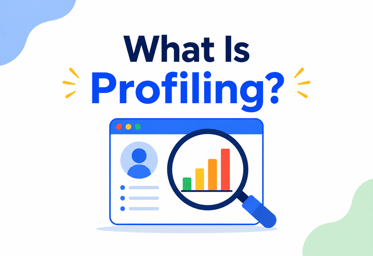
What Is Profiling?
A complete guide to understanding where your code really spends its time — from the first line-counting hacks of the 1970s to distributed, always-on profiling at Netflix and Google scale.
Introduction & History
Profiling is the practice of measuring a running program to find out exactly where it spends its time, memory, and other resources — a fitness tracker for your code, replacing intuition with evidence.
Think of a profiler like a fitness tracker for your code. Instead of guessing which part of your body worked hardest during a run, the tracker tells you precisely — “your legs did 70% of the work, your arms 10%.” A profiler does the same thing for a program, telling you “this function used 70% of the CPU time, this other one allocated 2 GB of memory.”
The word “profile” here means a shape or outline — in this case, the shape of how a program’s resources are used over time. When people ask “what is profiling?”, they are really asking: how do we see inside a running program without stopping it or rewriting it, so we can find the exact part that is slow, wasteful, or risky?
This terminology sometimes bleeds into security discussions too, because the word “profiling” is also used in security and data-privacy contexts to mean building a behavioural picture of a user or system (for example, “security profiling” of network traffic to detect anomalies). Both meanings share the same root idea: observe behaviour over time and build a picture of it. This guide focuses mainly on software performance profiling — the discipline every backend, systems, and platform engineer relies on — and dedicates a full chapter later to how the same ideas apply to security profiling.
A profiler is to code what a fitness tracker is to a runner — it does not change the workout, it just tells you honestly where the effort actually went.
A Short History of Profiling
1973 — gprof is born
Bell Labs built early call-graph profilers for Unix; gprof, released with BSD Unix in the early 1980s, became the standard tool for a generation of C programmers.
1990s — Sampling profilers arrive
Instead of instrumenting every function call (which slows a program down), sampling profilers began interrupting the CPU periodically and recording “what is running right now?” This drastically lowered overhead.
2000s — JVM & managed runtimes
Java’s JVM shipped built-in hooks (JVMTI) that let tools like JProfiler, YourKit, and VisualVM inspect a live application without modifying its code.
2014 — Flame graphs
Brendan Gregg popularised the flame graph, a visualisation that turned huge stacks of profiling data into an intuitive picture anyone could read in seconds.
2019 – today — Continuous profiling
Companies like Google (with its internal Google-Wide Profiling system) and later open-source tools (Pyroscope, Parca, async-profiler) made profiling something that runs all the time in production, not just when something breaks.
The Problem Profiling Solves
Software performance intuition is famously unreliable. Profiling is what replaces “I think this is slow” with “here is exactly where the time went.”
Imagine a delivery company whose trucks keep arriving late. The manager could guess (“maybe the drivers are slow,” “maybe the routes are bad”) or they could actually track each truck’s GPS and stopwatch every stage of the trip. Profiling is the GPS-and-stopwatch approach applied to software.
Without profiling, engineers fall back on intuition — and intuition about performance is famously unreliable. A method that looks slow because it has a nested loop might contribute almost nothing to total run time, while an innocent-looking database call might be responsible for 80% of a request’s latency. This mismatch between what looks slow and what is actually slow is why the famous saying exists: “premature optimisation is the root of all evil” — because engineers who optimise based on guesswork often optimise the wrong thing.
Profiling solves three concrete problems:
- Where is the time going? (CPU profiling) — which functions, queries, or requests consume the most processing time.
- Where is the memory going? (memory / heap profiling) — which objects are allocated, retained, or leaked.
- What is the system’s behavioural fingerprint? (security / behavioural profiling) — what does “normal” look like, so abnormal (an attack, a bug, a bot) stands out.
Profiling doesn’t make code faster. It tells you honestly which part is slow, so the fix — when it comes — lands on the part of the code that actually matters.
Core Concepts
Two collection strategies, half a dozen data flavours, and one universal visualisation — the vocabulary every profiler user needs.
Sampling vs. Instrumentation
There are two fundamentally different ways a profiler can gather data:
Sampling Profiler
- Periodically “wakes up” (e.g., 100 times per second) and records what the CPU is currently doing.
- Like a teacher glancing around the classroom every few seconds to see who’s talking — not perfectly precise, but very low overhead and statistically accurate over time.
- Examples:
async-profiler, Linuxperf, Google’s continuous profiler.
Instrumentation Profiler
- Inserts extra tracking code at the start and end of every function call, so it records every single call exactly.
- Like putting a timestamp stamper at every classroom door — perfectly precise, but changes behaviour and slows the program down significantly (sometimes 10–100×).
- Examples: JProfiler in instrumentation mode,
cProfilein Python.
Types of Profiling
CPU Profiling
Measures which code paths consume the most processor time. The most common type; answers “what is slow?”
Memory / Heap Profiling
Tracks object allocation and retention. Answers “what’s using RAM, and what’s leaking?”
Wall-clock vs. CPU-time
Wall-clock includes time spent waiting (I/O, locks); CPU-time only counts time actually executing on a core.
Lock / Contention Profiling
Finds threads blocked waiting for locks — a common hidden cause of latency in concurrent systems.
I/O Profiling
Measures time spent on disk reads, network calls, and database queries — often the true bottleneck in modern services.
Security / Behavioural Profiling
Builds a baseline “profile” of normal system or user behaviour to detect anomalies and threats.
Flame Graphs — the Universal Visualisation
A flame graph stacks function calls vertically (caller at the bottom, callee above) and sizes each box horizontally by how much time it consumed. It is not about left-to-right time order — it’s about width. A wide box near the top of the flame is almost always your bottleneck.
In this example, even though handleRequest() looks like the “main” function, the real bottleneck is connectionPool.wait() — the program is spending 40% of its time waiting for a free database connection, not doing actual work. This is exactly the kind of insight that raw intuition would miss.
Architecture & Components
Whether it’s a small local tool or a company-wide continuous profiler, every profiling system is built from the same handful of building blocks.
A typical profiling system is made of the same core parts, arranged in a pipeline that starts inside the running application and ends at a flame graph on an engineer’s screen.
| Component | What it does |
|---|---|
| Collector / Agent | Runs alongside the app (in-process or as a sidecar) and captures raw samples — stack traces, timestamps, thread IDs. |
| Symbolizer | Converts raw memory addresses or bytecode offsets into human-readable function names and line numbers. |
| Aggregator | Merges thousands of samples into a compact structure (like a call tree) instead of storing every raw sample forever. |
| Storage | A time-series or specialised profile store (e.g., Parquet-based, or purpose-built like Pyroscope’s storage engine). |
| Query & Visualisation Layer | Turns stored profiles into flame graphs, diff views (compare before / after a deploy), and top-N tables. |
How Profilers Work Internally
Under the hood, most modern sampling CPU profilers rely on a very small set of operating-system or runtime tricks — timer interrupts, stack walks, and aggregation.
Modern sampling profilers repeat four steps, thousands of times a second, and let statistics do the rest:
- Timer interrupt: The OS or runtime sets up a timer (e.g.,
setitimeron Linux, or a JVM safepoint mechanism) that fires many times per second. - Stack walk: On each interrupt, the profiler walks the current call stack — the chain of “who called whom” — from the currently executing function back up to
main(). - Record: That single stack trace is recorded as one “sample.”
- Repeat & aggregate: After thousands of samples, functions that appear more often in the samples are statistically the ones consuming more CPU time.
A sampling profiler is like a nature photographer taking a photo of a forest every second. No single photo tells the whole story, but after a thousand photos, you can clearly see which trees animals visit most often — even though nobody watched continuously.
A Minimal Instrumentation-Style Profiler in Java
To make this concrete, here’s a small, simplified example that manually times method calls. This is essentially what instrumentation profilers automate for you at scale — they inject the same “enter/exit” hooks into every method at load time.
public class SimpleProfiler {

    private static final ThreadLocal<Deque<Frame>> stack =
        ThreadLocal.withInitial(ArrayDeque::new);
    private static final Map<String, Long> totalNanos = new ConcurrentHashMap<>();

    record Frame(String name, long startNanos) {}

    public static void enter(String methodName) {
        stack.get().push(new Frame(methodName, System.nanoTime()));
    }

    public static void exit() {
        Frame f = stack.get().pop();
        long elapsed = System.nanoTime() - f.startNanos();
        totalNanos.merge(f.name(), elapsed, Long::sum);
    }

    public static void report() {
        totalNanos.entrySet().stream()
            .sorted((a, b) -> Long.compare(b.getValue(), a.getValue()))
            .forEach(e ->
                System.out.printf("%-30s %8.2f ms%n",
                    e.getKey(), e.getValue() / 1_000_000.0));
    }
}

// Usage inside business logic:
public class OrderService {
    public void processOrder(Order order) {
        SimpleProfiler.enter("processOrder");
        try {
            validate(order);
            charge(order);
            notifyWarehouse(order);
        } finally {
            SimpleProfiler.exit();
        }
    }
}
Real profilers do the same “enter / exit + accumulate” logic, but at the bytecode level (via javaagent instrumentation) or via kernel-level sampling — so you never have to hand-write this in production code.
Data Flow & Lifecycle
A profiling session, from the first timer interrupt to the final flame graph, follows a five-stage lifecycle that every tool implements in some form.
Data flows from the running application, through the collector, into storage, and finally out to the engineer inspecting a flame graph:
Key stages worth understanding individually:
- Capture: raw, cheap, in-process data collection.
- Buffer & batch: samples are held briefly and compressed before leaving the host, to avoid flooding the network.
- Symbolise: raw addresses become readable names — this can happen at capture time or later, depending on the tool.
- Aggregate: millions of samples collapse into a call tree with counts per function.
- Retain & expire: most systems keep high-resolution data for hours / days and downsampled data for weeks, similar to metrics retention policies.
Advantages, Disadvantages & Trade-Offs
Profiling is not free — and the choice between sampling and instrumentation is one of the most consequential decisions on the topic.
Advantages
- Replaces guesswork with data — you optimise what actually matters.
- Sampling profilers have very low overhead (often < 1–2%), safe for production.
- Flame graphs make huge amounts of data instantly readable.
- Continuous profiling lets you compare “before vs. after” a deploy automatically.
- Works across CPU, memory, locks, and I/O — one mental model, many resource types.
Disadvantages & Trade-Offs
- Instrumentation profilers can slow programs down dramatically — not safe for production use.
- Sampling has statistical blind spots for very short-lived functions (they may be sampled too rarely to appear).
- Symbolisation and storage at scale is a real engineering problem, not a solved one out of the box.
- Profiling data can be sensitive (it reveals code structure and sometimes business logic) — needs access control.
- Interpreting flame graphs correctly takes practice; misreading them leads to wrong conclusions.
Performance & Scalability
A slow profiler defeats its own purpose — it can even hide the real bottleneck by becoming one. Two dimensions of scale matter: per-host and fleet-wide.
1. Per-Host Overhead
Sampling frequency is the main lever. Sampling at 1000 Hz (1000 times a second) gives very precise data but costs more CPU; sampling at 19 Hz (a deliberately “odd,” non-round number used by many production profilers to avoid lock-step artefacts with other periodic system activity) is nearly invisible.
2. Fleet-Wide Scalability
Running a profiler on one server is easy. Running it continuously across 50,000 servers, storing months of history, and letting engineers query it in under a second is a distributed-systems problem in its own right — this is what makes Google-Wide Profiling and tools like Pyroscope / Parca notable engineering achievements, not just “a profiler.”
High Availability & Reliability
A profiling agent runs inside a production process. It has to be reliable enough that engineers forget it is there.
Because profiling agents run alongside real user traffic, reliability rules are strict — a buggy profiler must never be allowed to crash or destabilise the application it’s watching. Four design guarantees hold in every serious production profiler:
- Fail open, not closed: if the profiling agent errors, the application must keep running normally.
- Backpressure handling: if the storage backend is unreachable, agents buffer briefly then drop old data rather than consuming unbounded memory.
- Circuit breakers: automatic disabling of profiling if overhead crosses a safety threshold.
- Rolling deploys of the agent itself: profiler upgrades follow the same canary / rollback discipline as any other production service.
Security Profiling
The two meanings of “profiling” connect here: same technique — observe repeatedly, build a baseline — but a different question.
In security, profiling means building a baseline of what “normal” looks like for a system, network, or user — so that deviations can be flagged as potential threats. It borrows the exact same idea as performance profiling: observe behaviour repeatedly, build a statistical picture, and use that picture to spot outliers.
Network Traffic Profiling
Baselines typical request volume, source IPs, and protocols to detect DDoS attacks or data exfiltration.
User Behaviour Profiling
Learns a user’s typical login times and locations to flag account-takeover attempts before damage is done.
Application Security Profiling
Uses runtime profiling data (which code paths execute) to detect code injection or unexpected execution paths — a technique behind some Runtime Application Self-Protection (RASP) tools.
Side-Channel Risk
Because profilers observe fine-grained timing, poorly secured profiling data can itself leak sensitive information (timing side channels) — so profiling tools need their own access controls.
Performance profiling asks “where does time go?” to make software faster. Security profiling asks “does this behaviour match the normal baseline?” to catch threats. They share tooling concepts (sampling, baselining, anomaly detection) but serve different goals — don’t conflate a CPU flame graph with a security threat model.
Monitoring, Logging & Metrics
Profiling is the fourth pillar of observability. On its own it’s useful; correlated with the other three, it’s transformative.
Profiling is one of the four pillars of observability, alongside metrics, logs, and traces — each answers a different question about the same running system:
| Pillar | Answers | Granularity |
|---|---|---|
| Metrics | “Is something wrong right now?” (e.g., CPU at 95%) | Aggregated numbers over time |
| Logs | “What specific events happened?” | Discrete event records |
| Traces | “Which service in this request was slow?” | Per-request, cross-service |
| Profiles | “Which line of code inside that service was slow?” | Per-function, sub-request |
Modern observability platforms (Grafana + Pyroscope, Datadog Continuous Profiler, Google Cloud Profiler) let engineers click from a slow trace span directly into the flame graph for that exact time window — connecting “which service” to “which line of code” in one workflow.
Metrics tell you the room is on fire. Logs tell you what caught fire. Traces tell you which room. Profiles tell you which piece of furniture.
Deployment & Cloud
Where the agent runs is almost as important as what it collects. Three deployment models dominate modern profiling.
Profiling agents are typically deployed one of three ways:
- In-process library: a dependency added to the application (e.g.,
async-profilerattached via JVM agent flags). Simplest, but tied to the app’s lifecycle. - Sidecar container: in Kubernetes, a separate container in the same pod that attaches to the main process — common for language-agnostic profilers like
Parca Agentusing eBPF. - Node-level daemon (eBPF-based): a single agent per physical or virtual host profiles every process on that host using kernel-level eBPF hooks, requiring zero code changes — the modern standard for fleet-wide continuous profiling.
eBPF-based profilers are popular in Kubernetes because they need no code changes, no redeploys, and no per-language agents — one DaemonSet profiles every pod on a node regardless of whether it’s written in Java, Go, Python, or Rust.
Databases, Caching & Load Balancing
The same profiling principles apply to the data tier — SQL, caches, and load balancers all have their own profilers, whether they’re marketed that way or not.
Profiling isn’t just for application code. The same “observe, aggregate, visualise” loop is at the heart of every good data-layer tool:
- Database query profiling: tools like
EXPLAIN ANALYZE(Postgres) or the MySQL slow query log are, in effect, specialised profilers for SQL execution plans. - Cache hit / miss profiling: tracking which cache keys are hot vs. cold helps size caches correctly and choose eviction policies.
- Load balancer profiling: observing request latency distribution per backend node reveals uneven load (“hot” instances) that a round-robin balancer might be masking.
A profiling storage backend itself is usually built on the same technology it helps others optimise: time-series databases or columnar stores (like Parquet) chosen specifically because profile data is write-heavy, append-only, and queried by time range — a workload that cache-and-database engineers will recognise immediately.
APIs & Microservices
A single user request can touch a dozen services. Profiling extends naturally into that world when it’s tied to distributed tracing.
In a microservices architecture, one incoming request often fans out across auth, product, order, and payment services before returning a response. Distributed profiling stitches per-service profiles together using trace IDs, so engineers can follow a slow request from its entry point down to the exact function that made it slow.
When a trace shows the Payment Service took 400 ms of a 500 ms total request, an engineer can pivot directly into that service’s profile for the exact timestamp and see the specific function (e.g., a JSON serialisation call, or a synchronous network call) responsible — without needing to reproduce the issue locally.
Design Patterns & Anti-Patterns
A short list of habits that separate teams who profile occasionally from teams who use profiling as an engineering practice.
Good Patterns
- Continuous, always-on profiling at low sampling rates, rather than only profiling when something is already on fire.
- Diff profiling: comparing a flame graph before and after a code change or deploy to catch regressions automatically.
- Correlate profiles with traces / metrics instead of viewing them in isolation.
Anti-Patterns
Performance characteristics under real production traffic, real data volumes, and real concurrency are often completely different from staging — leading engineers to “fix” the wrong bottleneck.
One flame graph can be a statistical fluke. Look at trends over multiple runs and time windows before drawing conclusions.
Leaving a full instrumentation profiler running against live traffic is the single most common cause of “the profiler made things worse” incidents.
Best Practices & Common Mistakes
Do these, avoid those — a working checklist for teams introducing profiling to a real codebase.
Best Practices
- Prefer sampling profilers for anything running in production.
- Profile under realistic load, not synthetic idle conditions.
- Always look at both CPU and wall-clock time — a function can be “fast” on CPU but slow overall due to waiting.
- Store and version profiles alongside deploys so regressions are traceable to a specific commit.
- Restrict access to profiling data the same way you would logs — it can reveal sensitive logic.
Common Mistakes
- Assuming the function that looks complex is the bottleneck without measuring.
- Ignoring lock contention and I/O wait, focusing only on raw CPU-bound code.
- Profiling once and never again — performance regresses silently over time as code changes.
- Confusing security “profiling” (behavioural baselining) with performance profiling and applying the wrong tool.
Real-World Examples
How the largest engineering organisations in the world put continuous profiling to work in production.
Google-Wide Profiling
A continuous, fleet-scale sampling profiler running across essentially all of Google’s production machines, published in a well-known 2010 research paper, credited with finding compiler- and library-level optimisations worth enormous aggregate CPU savings.
JVM at Streaming Scale
Uses Java Flight Recorder and async-profiler extensively to tune JVM services handling massive streaming traffic, and has published widely on flame-graph-driven performance work.
Continuous Profiling in CI/CD
Runs continuous profiling across its microservices fleet to catch performance regressions automatically as part of the CI / CD pipeline, tying profiles directly to deploys.
AWS CodeGuru Profiler
AWS offers CodeGuru Profiler as a managed service, specifically marketed around finding the exact expensive lines of code in production applications with low overhead.
Frequently Asked Questions
Short answers to the questions engineers ask most often when profiling comes up for the first time.
Is profiling the same as debugging?
No. Debugging finds why something is incorrect (a bug). Profiling finds where resources are spent, even when the program is working correctly — it’s about performance, not correctness.
Does profiling slow my application down?
Sampling profilers add very little overhead (often under 1–2%) and are considered safe for production. Instrumentation profilers can add significant overhead and are generally reserved for local development or short diagnostic sessions.
What’s the difference between profiling and tracing?
Tracing follows one request across multiple services to show where time went between services. Profiling zooms into one process to show where time went between functions and lines of code. They complement each other.
Why is security sometimes discussed alongside profiling?
Because the underlying technique — observing behaviour repeatedly to build a baseline and spot deviations — is shared between performance profiling (spotting slow code) and security profiling (spotting anomalous, potentially malicious behaviour). They use similar statistical tools but answer different questions.
What tools should I start with?
For Java: async-profiler or Java Flight Recorder. For Python: py-spy. For Go: pprof (built into the standard library). For a fleet-wide, always-on setup: Pyroscope or Parca, both open source.
Summary & Key Takeaways
Six ideas from this guide worth carrying with you into every performance conversation.
Remember This
- Profiling replaces guesswork with data. It measures where a running program actually spends CPU time, memory, and other resources.
- Sampling profilers belong in production. They are low-overhead and safe; instrumentation profilers are precise but expensive, and are best kept for development.
- Flame graphs are the standard visualisation. Width means time spent, not left-to-right order. A wide box near the top is almost always your bottleneck.
- Profiling is the fourth pillar of observability. Alongside metrics, logs, and traces, it works best when correlated with the others.
- Security “profiling” shares the same core idea — a behavioural baseline. But it serves a different purpose: detecting anomalies and threats, not optimising performance.
- Modern practice favours continuous profiling. Always-on, fleet-wide (often via eBPF), instead of one-off manual sessions triggered only after something breaks.