What Is an Index in a Database?
A complete, book‑quality walkthrough — from the librarian’s card catalog to how Netflix, Amazon, and Uber keep billion‑row tables fast. No prior knowledge required.
Introduction & History
Imagine you walk into a library with 2 million books and no card catalog, no shelf labels, and no way to search anything. You are looking for one specific book: “The Old Man and the Sea.” The only way to find it is to start at the first shelf and read the title of every single book, one at a time, until you find it — or reach the end and discover it isn’t there at all.
That is exactly what a database does every time it looks for data, unless it has an index.
A database index is a separate, organized data structure that a database keeps next to your actual data, whose only job is to help the database find rows quickly — without having to look at every single row. It is one of the oldest, simplest, and most powerful ideas in all of computer science, and it is arguably the single most important tool a software engineer can master to make an application fast.
A Short History
The idea of an “index” did not start with computers. Libraries have used card catalogs since the 1870s — a separate cabinet of small cards, sorted alphabetically by author or title, each card pointing to a shelf location. You didn’t have to search the whole library; you searched a small, sorted catalog instead, and it told you exactly where to walk.
When relational databases were invented in the early 1970s (IBM’s System R, and later Oracle, Ingres, and DB2), engineers faced the exact same problem at a much larger scale — millions of rows instead of thousands of books. They borrowed data structures from computer science research: notably the B‑Tree, invented by Rudolf Bayer and Edward McCreight at Boeing Research Labs in 1970. The B‑Tree (and its later variant, the B+Tree) turned out to be almost perfectly suited to how disks store data, and it remains — more than 50 years later — the backbone of indexing in almost every relational database on Earth: MySQL, PostgreSQL, Oracle, SQL Server, and even many NoSQL databases like MongoDB.
Library card catalogs
Libraries adopt separate cabinets of small alphabetically‑sorted cards, each pointing to a shelf location — the earliest “index,” four generations before computers.
The B‑Tree is born
Rudolf Bayer and Edward McCreight publish the B‑Tree at Boeing Research Labs — a structure engineered for how disks read data in pages, still the backbone of database indexing today.
Relational databases
IBM’s System R, then Oracle, Ingres and DB2 apply B‑Trees to millions of rows, making SQL commercially viable and inventing the query optimizer that decides when to use them.
B+Tree everywhere
MySQL, PostgreSQL and SQL Server standardize on the B+Tree variant — leaf‑only data pointers and linked leaves — because it makes range scans dramatically faster.
NoSQL borrows the idea
MongoDB, Cassandra and DynamoDB carry the indexing concept into distributed key‑value and document models — different structures, same core mission of avoiding full scans.
Specialized indexes
Hash, bitmap, inverted (Elasticsearch, Google), spatial (Uber, Airbnb) and vector (AI similarity) indexes solve variations of the same problem: how do you find something fast in a huge pile of data without checking everything?
A database without an index is a library where books are thrown onto shelves in the order they arrived, with no catalog. A database with an index is that same library, but now there’s a card catalog sorted by title, sitting in a small cabinet near the entrance, so you can find any book’s exact shelf location in seconds.
Today, indexing has grown far beyond a single data structure. Modern databases use B+Trees, hash indexes, bitmap indexes, inverted indexes (used by search engines like Elasticsearch and Google), spatial indexes (for maps and geolocation, used by Uber), and vector indexes (for AI similarity search, used by recommendation engines). But they are all solving the exact same core problem this tutorial is about: how do you find something fast, in a huge pile of data, without checking everything?
The Problem & Motivation
Let’s make this concrete. Suppose you have a table called users with 10 million rows, and you run this query:
SELECT * FROM users WHERE email = 'alice@example.com';Without an index, the database engine has exactly one option: read every single row in the table, check if its email column matches, and keep or discard it. This is called a full table scan. If the row you want happens to be the very last one checked, the database has done 10 million comparisons for one answer.
A full table scan has a time complexity of O(n) — the time it takes grows in direct, linear proportion to the number of rows. Double the rows, double the time. At 10 rows this is invisible. At 10 million rows, it can mean a query that takes 8 seconds instead of 2 milliseconds — a 4,000× difference — which is the difference between an app that feels instant and one that makes users close the tab.
Where This Problem Shows Up in Real Life
- E‑commerce: Amazon needs to find a specific order by order ID among billions of orders, instantly, every time someone checks their order status.
- Social media: Instagram needs to load “posts by user X” out of billions of posts, in under 100 milliseconds, for every profile view.
- Banking: A bank needs to find “all transactions for account #123456” out of trillions of transaction records, without scanning the whole ledger.
- Ride‑hailing: Uber needs to find “drivers near this location” out of millions of active drivers, in real time.
Every one of these scenarios would be completely impossible at scale without indexing. This is not an optimization — it is a foundational requirement for building any application that has to serve real users with real data volumes.
Visualizing the Problem
That difference — O(n) versus O(log n) — is the entire reason indexes exist. We’ll unpack exactly what “O(log n)” means and how it’s achieved in the next sections.
Core Concepts
Before going deeper, let’s pin down exactly what an index is, how it’s described, and the vocabulary you’ll see repeated in every real database.
3.1 What Is an Index?
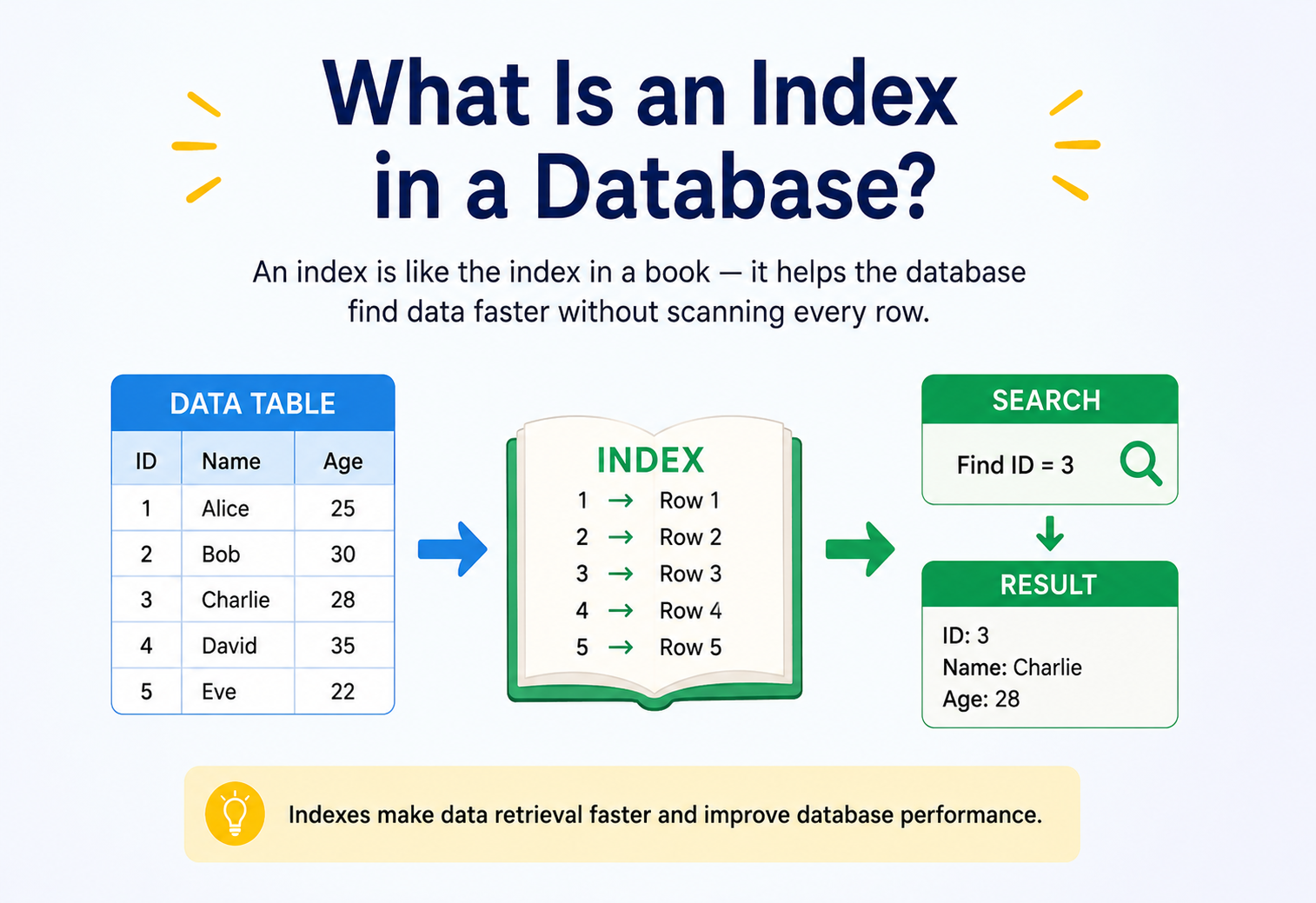
A database index is a data structure — usually a sorted, tree‑shaped structure — built on one or more columns of a table. It stores the column’s values along with a pointer to where the full row lives on disk. Instead of searching the whole table, the database searches this small, sorted structure, finds the pointer, and jumps directly to the row.
A sorted lookup structure
A separate, smaller, sorted copy of one or more columns from your table, plus a pointer back to the original row, organized in a structure that supports fast searching.
Avoid scanning every row
To avoid scanning every row when the database needs to find, sort, filter, or join data — turning slow O(n) searches into fast O(log n) searches.
Everywhere
Every relational database (MySQL, PostgreSQL, Oracle, SQL Server), most NoSQL databases (MongoDB, Cassandra, DynamoDB), search engines (Elasticsearch), and even in‑memory data stores.
The back‑of‑book index
Think of the index at the back of a textbook. If you want to find every page that mentions “photosynthesis,” you don’t read all 400 pages — you flip to the index at the back, find “photosynthesis,” and it tells you: pages 45, 112, 230. You jump straight there.
CREATE INDEX idx_users_email ON users(email);This single line tells the database: “Build a sorted structure of every email value in the users table, each pointing back to its row. From now on, use it whenever a query filters or sorts by email.”
3.2 The Book Index Analogy, Fully Explained
Let’s go deeper on this analogy because it is genuinely the best mental model for understanding indexes, and it works whether you’re 10 years old or a senior engineer.
- The book’s pages = the actual table (called the “heap” or “table data”) — the real content, stored in the order it was written.
- The index at the back of the book = the database index — a much smaller, alphabetically sorted list of important words, each with page numbers.
- Looking up a word in the index, then flipping to the page = the database using the index to find a pointer, then fetching the row.
- The index doesn’t contain the whole page’s content — just the word and the page number. Similarly, a database index usually doesn’t store the whole row — just the indexed column(s) and a pointer.
3.3 Key Terminology
| Term | Meaning |
|---|---|
Table / Heap | The actual storage location of your rows, usually unordered or ordered by insertion. |
Index | A separate sorted structure pointing back to rows. |
Key | The column (or columns) the index is built on, e.g., email. |
Pointer / Row ID (RID) | A reference telling the database exactly where the actual row lives on disk. |
Full Table Scan | Reading every row to find matches — what happens without an index. |
Index Seek / Lookup | Directly navigating to the matching entry using the index structure. |
Selectivity | How unique a column’s values are. High selectivity (like an email) makes a great index; low selectivity (like a boolean “is_active”) usually doesn’t. |
Cardinality | The number of distinct values in a column. |
3.4 Why Not Just Index Everything?
A natural question: if indexes make reads faster, why not put an index on every column? We’ll explore this in depth in Chapter 09, but the short answer is that every index has to be updated whenever you insert, update, or delete a row — so more indexes means slower writes, more disk space, and more maintenance overhead. Indexing is always a trade‑off between read speed and write speed.
Architecture & Components
An index is not one single thing — it’s a system made of several components working together. Let’s break down the architecture piece by piece.
4.1 The Two Storage Layers
- The Table (heap or clustered store): Where the actual row data lives — every column, every byte.
- The Index: A smaller structure containing only the indexed column(s) plus a pointer back to the matching row in the table.
4.2 Pages and Blocks
Databases don’t read data one row at a time from disk — that would be far too slow. Instead, they read fixed‑size chunks called pages (typically 8 KB in PostgreSQL, 16 KB in MySQL InnoDB). Both the table and the index are organized into pages. This matters because it directly shapes how index structures like the B+Tree are designed — each “node” of the tree is sized to fit neatly into one page, so that reading one tree node means exactly one disk read.
4.3 Core Components of a B+Tree Index
| Component | Role |
|---|---|
| Root node | The single entry point at the top of the tree; every search starts here. |
| Internal (branch) nodes | Store ranges of key values and pointers to child nodes — they guide the search downward. |
| Leaf nodes | The bottom level; store the actual key values and pointers to rows (or the rows themselves, in a clustered index). Leaf nodes are linked together in a chain for fast range scans. |
| Pointers / row locators | References that tell the database exactly where to find the real row — either a physical disk address or, in some databases, the primary key value. |
4.4 Where Indexes Live in the Overall Database Architecture
Having an index does not guarantee the database will use it. The query optimizer estimates the cost of each possible execution plan and picks the cheapest one. If a table is tiny, or if a query would return most of the table anyway, a full scan can actually be faster than using the index — because jumping around a B+Tree involves more scattered disk reads than reading the table sequentially.
Internal Working — The B+Tree Deep Dive
The B+Tree is, by far, the most common index structure in production databases. Let’s understand exactly how it works, step by step.
5.1 Why a Tree, and Why “B”?
A simple binary search tree (each node has at most 2 children) would technically work, but it would be too “tall” — for a million rows, you’d need about 20 levels, and each level might mean a separate disk read, which is slow (disk reads are roughly 100,000 times slower than memory reads).
A B‑Tree solves this by allowing each node to have many children — often hundreds — not just two. This makes the tree extremely “wide and short” (called a low fan‑out height) instead of tall and thin. For a million rows with a fan‑out of 500, you need only about 3 levels to reach any row. That means only 3 disk reads to find any single record among a million — and modern databases cache the top levels in memory, often reducing this to a single physical disk read.
Think of the difference between a corporate org chart where every manager has only 2 direct reports (you’d need many layers to reach 1,000 employees) versus one where every manager has 20 direct reports (you’d only need 3 layers). B‑Trees are “flat, wide org charts” for data.
5.2 B‑Tree vs. B+Tree
Most real databases actually use a B+Tree, a refinement of the original B‑Tree:
- In a B‑Tree, data pointers can live in internal nodes as well as leaf nodes.
- In a B+Tree, all actual data pointers live only in the leaf nodes. Internal nodes hold only keys used for navigation — no data.
- Leaf nodes in a B+Tree are linked together in a chain (a doubly linked list), which makes range queries (
WHERE age BETWEEN 20 AND 30) extremely fast — you find the starting leaf once, then simply walk sideways along the chain.
5.3 Step‑by‑Step: How a Search Works
Let’s trace a search for the value 72 in a B+Tree index on an age column.
- Start at the root. The root holds a small number of separator keys, e.g.,
[30, 60, 90]. The database compares 72 against these and determines it lies between 60 and 90. - Follow the correct pointer down to the branch node responsible for the range 60–90.
- Repeat at the branch level — this node might have separators like
[65, 75, 85]. Since 72 is between 65 and 75, follow that pointer. - Arrive at a leaf node. The leaf contains actual sorted key values (e.g., 70, 71, 72, 73) each paired with a pointer to the real row.
- Follow the pointer to fetch the actual row from the table.
5.4 The Math: Why O(log n) Is So Powerful
With a fan‑out of about 500 per node (realistic for an 8 KB page holding small integer keys), here’s how many levels you need for different table sizes:
| Rows in table | Full scan comparisons | B+Tree levels needed |
|---|---|---|
| 1,000 | 1,000 | 1 |
| 1,000,000 | 1,000,000 | ~3 |
| 1,000,000,000 | 1,000,000,000 | ~4 |
This is the entire reason a query on a billion‑row table can still return in milliseconds: instead of a billion comparisons, the database does about four.
5.5 Other Internal Structures: Hash Indexes
Not every index is a tree. A hash index runs the key through a hash function that converts it into a fixed‑size number, which is used to directly locate a “bucket” containing the pointer. This gives true O(1) — constant time — lookups for exact‑match queries (WHERE id = 5), even faster than a B+Tree in theory.
However, hash indexes cannot support range queries (WHERE age BETWEEN 20 AND 30) or sorting, because hashing deliberately scrambles the order of values. This is why B+Trees remain the default choice for general‑purpose indexing, while hash indexes are used in more specialized situations (like PostgreSQL’s HASH index type, or in‑memory key‑value stores like Redis).
Types of Database Indexes
The B+Tree is the most common structure, but real databases layer many flavours of index on top of it — each optimised for a different query shape.
6.1 Clustered Index
A clustered index determines the physical order in which rows are stored on disk. There can be only one clustered index per table, because rows can only be physically sorted one way. In many databases (like SQL Server and MySQL’s InnoDB engine), the primary key automatically becomes the clustered index, and the leaf nodes of the B+Tree are the actual table rows — not just pointers to them.
A clustered index is like a dictionary: the words themselves are physically arranged in alphabetical order on the page. There’s no separate lookup step — the “index” and the “data” are the same physical arrangement.
6.2 Non‑Clustered (Secondary) Index
A non‑clustered index is a separate structure from the table. Its leaf nodes store the key value plus a pointer (in InnoDB, this pointer is the primary key value; in other engines, it might be a physical row address). You can have many non‑clustered indexes on one table.
This is the book‑index‑at‑the‑back‑of‑the‑book scenario: a completely separate, sorted list with page‑number pointers, distinct from the actual pages.
6.3 Unique Index
Enforces that no two rows can have the same value in the indexed column(s), while also speeding up lookups. Primary keys automatically get a unique index; you can also create one manually (e.g., on an email column to prevent duplicate signups).
CREATE UNIQUE INDEX idx_unique_email ON users(email);6.4 Composite (Multi‑Column) Index
An index built across more than one column, e.g., (last_name, first_name). Order matters enormously here — a composite index is only efficient for queries that filter using a “leftmost prefix” of the columns.
CREATE INDEX idx_name ON employees(last_name, first_name);

-- Uses the index efficiently:
SELECT * FROM employees WHERE last_name = 'Smith';
SELECT * FROM employees WHERE last_name = 'Smith' AND first_name = 'Anna';

-- Does NOT use the index efficiently (first_name is not the leftmost column):
SELECT * FROM employees WHERE first_name = 'Anna';Think of a phone book sorted by (last name, then first name). You can quickly find all “Smiths,” and within that, quickly find “Smith, Anna.” But you cannot quickly find everyone with the first name “Anna” — you’d have to scan every Smith, every Jones, every Lee, etc.
6.5 Covering Index
A special case where the index contains every column a query needs, so the database never has to touch the actual table at all — it answers entirely from the index. This is sometimes called an “index‑only scan.”
CREATE INDEX idx_covering ON orders(customer_id, order_date, total_amount);

-- This query is fully answered by the index alone:
SELECT order_date, total_amount FROM orders WHERE customer_id = 42;
6.6 Full‑Text Index
Optimized for searching words within large text fields (e.g., blog posts, product descriptions). Instead of indexing whole column values, it indexes individual words, similar to how a search engine works. Used heavily by MySQL’s FULLTEXT index and dedicated engines like Elasticsearch.
6.7 Bitmap Index
Instead of a tree, this uses a bitmap (a string of 0s and 1s) per distinct value, where each bit represents whether a row has that value. Extremely efficient for columns with very few distinct values (low cardinality), like gender or order_status, and very common in analytical/data‑warehouse databases like Oracle and Amazon Redshift.
6.8 Spatial Index
Built for geographic and geometric data (points, lines, polygons), using structures like R‑Trees. This is what powers “find restaurants within 2 km” or “find the nearest available driver” queries — used extensively by Uber, Google Maps, and Airbnb.
6.9 Comparison Table
| Index type | Best for | Weakness |
|---|---|---|
| Clustered (B+Tree) | Primary key lookups, range scans | Only one per table; slower inserts if key isn’t sequential |
| Non‑Clustered (B+Tree) | Secondary lookups, sorting, filtering | Extra lookup step to fetch full row |
| Hash | Exact‑match lookups | No range queries, no sorting |
| Composite | Multi‑column filters | Column order matters strictly |
| Covering | Read‑heavy, index‑only queries | Larger index size |
| Full‑Text | Text/word search | Not for exact structured matches |
| Bitmap | Low‑cardinality analytics | Poor for high‑write OLTP systems |
| Spatial (R‑Tree) | Location/geometry queries | Specialized, not general‑purpose |
Data Flow & Lifecycle
An index isn’t a one‑time snapshot — it has to stay in sync with the table forever, through every insert, update, and delete. Let’s walk through what happens during each operation.
7.1 INSERT
- The new row is written into the table (heap or clustered structure).
- For every index defined on the table, the database computes the new key value and inserts it into the correct position in that index’s tree — which may require splitting a full leaf node into two.
7.2 UPDATE
- If the update changes an indexed column, the database must remove the old key entry from the index and insert the new one — effectively a delete + insert inside the index.
- If the update only touches non‑indexed columns, indexes on those columns are untouched (a good reason to index only what you truly query on).
7.3 DELETE
- The row is removed (or marked for removal) from the table.
- The corresponding entry is removed from every index. In practice, many databases perform a “lazy delete” — marking the entry as deleted and cleaning it up later in a background process — to avoid slowing down the delete operation itself.
This is why tables with 10 indexes are much slower to write to than tables with 1 or 2. Every INSERT becomes 11 writes instead of 1 (one to the table, ten to the indexes). This is the central trade‑off of indexing: faster reads, slower writes.
7.4 Page Splits — A Deeper Look
When a B+Tree leaf node fills up and a new key needs to be inserted, the database performs a page split: it creates a new leaf page, moves roughly half the entries into it, and updates the parent node’s pointers. If the parent node is also full, the split can cascade upward, occasionally all the way to the root — which is the one case where the tree grows an extra level. Page splits are a normal, expected part of index life, but excessive splitting (from random‑order inserts, discussed in Chapter 10) can cause fragmentation and hurt performance over time, which is why databases provide index rebuild/reorganize operations.
Java Code Examples
Below are practical, minimal Java (JDBC) examples showing how indexes are created and how their effect can be observed. These use plain JDBC so the concepts are visible without a framework layer in the way.
8.1 Creating an Index
import java.sql.Connection;
import java.sql.DriverManager;
import java.sql.Statement;

public class CreateIndexExample {
    public static void main(String[] args) throws Exception {
        String url = "jdbc:postgresql://localhost:5432/shopdb";
        try (Connection conn = DriverManager.getConnection(url, "app_user", "secret");
             Statement stmt = conn.createStatement()) {

            // A composite index supporting queries filtered by customer_id
            // and sorted/filtered further by order_date.
            stmt.execute(
                "CREATE INDEX IF NOT EXISTS idx_orders_customer_date " +
                "ON orders(customer_id, order_date)"
            );

            System.out.println("Index created successfully.");
        }
    }
}
8.2 Comparing Query Time With and Without an Index
import java.sql.*;

public class IndexPerformanceDemo {
    public static void main(String[] args) throws Exception {
        String url = "jdbc:postgresql://localhost:5432/shopdb";
        try (Connection conn = DriverManager.getConnection(url, "app_user", "secret")) {

            String query = "SELECT * FROM orders WHERE customer_id = ?";

            long start = System.nanoTime();
            try (PreparedStatement ps = conn.prepareStatement(query)) {
                ps.setInt(1, 42);
                try (ResultSet rs = ps.executeQuery()) {
                    int count = 0;
                    while (rs.next()) count++;
                    System.out.println("Rows found: " + count);
                }
            }
            long elapsedMs = (System.nanoTime() - start) / 1_000_000;
            System.out.println("Query time: " + elapsedMs + " ms");
        }
    }
}
Running this before and after creating idx_orders_customer_date on a large table typically shows a dramatic difference — often from hundreds of milliseconds down to single‑digit milliseconds.
8.3 Inspecting the Query Plan (Confirming Index Usage)
import java.sql.*;

public class ExplainPlanExample {
    public static void main(String[] args) throws Exception {
        String url = "jdbc:postgresql://localhost:5432/shopdb";
        try (Connection conn = DriverManager.getConnection(url, "app_user", "secret");
             Statement stmt = conn.createStatement();
             ResultSet rs = stmt.executeQuery(
                 "EXPLAIN ANALYZE SELECT * FROM orders WHERE customer_id = 42")) {

            while (rs.next()) {
                System.out.println(rs.getString(1));
            }
            // Look for "Index Scan using idx_orders_customer_date"
            // vs. "Seq Scan on orders" in the output.
        }
    }
}If the plan says Index Scan or Index Only Scan, the database used your index. If it says Seq Scan (sequential scan), it chose a full table scan instead — meaning either the index is missing, unused because of low selectivity, or the optimizer decided a scan was actually cheaper for this specific query.
8.4 A Simplified B+Tree Node in Java (For Learning)
This is a simplified, educational illustration of how a B+Tree leaf node might be represented in memory — not production code, but useful for building intuition about the structure discussed in Chapter 05.
import java.util.TreeMap;

public class SimpleBTreeLeafNode {
    // Sorted map: key value -> pointer to the row (e.g., a row ID or file offset)
    private final TreeMap<Integer, Long> entries = new TreeMap<>();
    private static final int MAX_ENTRIES = 4; // small on purpose, for illustration

    public void insert(int key, long rowPointer) {
        entries.put(key, rowPointer);
        if (entries.size() > MAX_ENTRIES) {
            splitNode();
        }
    }

    private void splitNode() {
        System.out.println("Leaf full - splitting node and promoting a key upward.");
        // In a real engine: create a sibling node, move half the entries,
        // and insert a separator key into the parent node.
    }

    public Long search(int key) {
        return entries.get(key); // O(log n) within the node
    }
}Advantages, Disadvantages & Trade‑offs
Indexes are one of the most powerful tools in a database engineer’s belt — and one of the most abused. Being honest about both sides keeps you from over‑ or under‑indexing.
Advantages
- Dramatically faster reads — turns O(n) scans into O(log n) lookups.
- Efficient sorting — an index already stores data in sorted order, so
ORDER BYcan often skip a separate sort step entirely. - Faster joins — joining two tables is much faster when the join column is indexed on at least one side.
- Enforces constraints — unique indexes prevent duplicate values automatically.
- Enables range queries — B+Tree indexes make “between,” “greater than,” and “less than” queries efficient.
Disadvantages
- Slower writes — every insert, update, or delete has to update every relevant index.
- Extra storage — indexes consume disk space, sometimes as much as (or more than) the table itself.
- Maintenance overhead — indexes can become fragmented over time and may need periodic rebuilding.
- Diminishing/negative returns if misused — indexing low‑selectivity columns, or too many columns, can actually hurt performance without helping any query.
9.3 The Core Trade‑off, Visualized
9.4 When NOT to Index a Column
| Situation | Why indexing doesn’t help |
|---|---|
| Very small tables (a few hundred rows) | A full scan is already fast; index overhead isn’t worth it. |
| Low‑selectivity columns (e.g., boolean flags) | Too many matching rows — the optimizer will likely ignore the index anyway. |
Columns rarely used in WHERE, JOIN, or ORDER BY | The index adds write cost with no read benefit. |
| Write‑heavy tables (e.g., high‑frequency logging tables) | Every extra index directly slows down every insert. |
| Columns that change frequently | Constant index updates add overhead disproportionate to any read gain. |
Performance & Scalability
Once you know what an index is, the next question is: how do you make sure yours actually stay fast as the data grows? A handful of concepts do most of the heavy lifting.
10.1 Index Selectivity and Cardinality
Selectivity is the ratio of distinct values to total rows. A column like email (nearly every value unique) has high selectivity and is an excellent index candidate. A column like gender (2–3 distinct values across millions of rows) has very low selectivity, and indexing it usually doesn’t help — the optimizer will often prefer a full scan anyway, since the index would still point to a huge fraction of the table.
10.2 Composite Index Column Order
As covered in Section 6.4, the order of columns in a composite index determines which queries can use it efficiently. A good rule of thumb: put the most selective and most frequently filtered column first, unless a specific query pattern demands otherwise. Many teams use the mnemonic “Equality, Sort, Range” — put equality‑filter columns first, then columns used for sorting, then range‑filter columns last.
10.3 Index Fragmentation and Random Inserts
If a table’s primary key is randomly generated (like a UUID) rather than sequential (like an auto‑incrementing integer), inserts land in random positions across the B+Tree instead of always appending at the end. This causes frequent page splits scattered throughout the tree, leading to fragmentation — pages that are only partially full, wasting space and slowing down range scans. This is why many high‑throughput systems prefer sequential IDs (or “sortable” UUIDs like UUIDv7) for primary keys when write throughput matters.
10.4 Covering Indexes for Read‑Heavy Workloads
As covered in Section 6.5, a covering index avoids the extra “index → table” hop entirely. On read‑heavy, latency‑sensitive systems (like a product catalog page), this technique alone can cut response times significantly, because the database never has to touch the (much larger, less cache‑friendly) table data.
10.5 Index Size vs. Cache (Buffer Pool)
Databases keep frequently accessed pages in memory (the “buffer pool” or “page cache”). If your indexes are small enough to fit entirely in memory, lookups become extremely fast because no disk I/O is needed at all. If indexes grow too large to fit in memory, the database starts evicting pages and re‑reading them from disk, which is far slower. This is a direct, practical reason to avoid indexing columns you don’t need — every unnecessary index competes for the same limited cache space.
10.6 Scalability: Indexes in Sharded / Distributed Databases
In a horizontally sharded system (data split across many database servers, common at companies like Uber and Instagram), each shard maintains its own local indexes. A query that filters by the shard key can go directly to the right shard and use its local index — fast. A query that filters by a non‑shard‑key column may have to broadcast the query to every shard (a “scatter‑gather” query), each using its local index, then merge results — which is much more expensive. This is why choosing the right shard key, in coordination with expected query patterns and indexes, is one of the most important decisions in distributed database design.
High Availability & Reliability
In production, indexes must stay healthy across crashes, replication, rebuilds, and disaster recovery. Their behaviour under these conditions is worth understanding explicitly.
11.1 Indexes and Replication
In a replicated database setup (one primary, multiple read replicas — used by nearly every large‑scale system, including Netflix and Amazon), indexes are typically replicated along with the table data itself, either via physical replication (copying the actual index pages) or logical replication (replaying the same DDL/DML statements, which rebuilds indexes independently on each replica). This means every replica must do the same index‑maintenance work on every write, which is one reason write‑heavy workloads don’t scale simply by adding more read replicas — the primary still bears the full indexing cost.
11.2 Index Corruption and Recovery
Indexes can, in rare cases, become corrupted — due to crashes, disk failures, or bugs. Because an index is a derived structure (it can always be recomputed from the table data), the standard recovery approach is to drop and rebuild the corrupted index rather than trying to repair it in place. Most production databases provide commands for this:
-- PostgreSQL
REINDEX INDEX idx_orders_customer_date;

-- MySQL
ALTER TABLE orders DROP INDEX idx_orders_customer_date,
                    ADD INDEX idx_orders_customer_date (customer_id, order_date);
11.3 Online Index Builds
Building or rebuilding an index on a large, live production table used to require locking the table (blocking all writes) for the duration — unacceptable for systems that can’t afford downtime. Modern databases solve this with online (concurrent) index builds, which allow writes to continue during index creation by tracking changes that happen mid‑build and applying them afterward.
-- Build without locking the table for writes
CREATE INDEX CONCURRENTLY idx_orders_customer_date ON orders(customer_id, order_date);Concurrent/online index builds take longer and use more resources than a locking build, and — in PostgreSQL specifically — they cannot run inside a transaction block. Always test the impact on a staging environment before running large index builds on production, and schedule them during lower‑traffic windows when possible.
11.4 Disaster Recovery
Because indexes are derivable from table data, backup strategies generally focus on backing up the table data (and often the index data too, for faster restore) as part of full database backups or snapshots. After a restore, if index data wasn’t included or is suspect, a full REINDEX pass guarantees correctness at the cost of rebuild time — a trade‑off disaster recovery runbooks need to account for explicitly.
Security
Indexes don’t enforce access control — but they interact with it in ways that matter to security engineers.
12.1 Indexes Don’t Enforce Access Control — But They Interact With It
Indexes themselves don’t decide who can read what; that’s the job of database permissions, row‑level security policies, and application‑layer authorization. However, indexes have real security‑relevant side effects worth knowing:
- Timing side‑channels: Because indexed lookups are much faster than unindexed ones, response‑time differences can sometimes leak information about whether a value exists (e.g., “does this email already exist?” answered near‑instantly via a unique index vs. slowly otherwise) — relevant in security‑sensitive systems like authentication, where such timing differences have historically been exploited to enumerate valid usernames.
- Sensitive data in indexes: An index built on a sensitive column (like a national ID number or an unhashed password — which should never happen) duplicates that data into another structure on disk, effectively widening the “attack surface” for anyone who gains raw file‑system or backup access.
- Query plan exposure: Verbose
EXPLAINoutput, exposed to end users or logged carelessly, can reveal internal schema and indexing details useful to an attacker probing a system — a reason to restrict query‑plan visibility to trusted internal tooling.
12.2 Best Practices
- Never index raw sensitive data (e.g., plaintext passwords, unencrypted card numbers). Encrypt or hash sensitive columns before storing/indexing them; index the hash, not the raw value, if lookups are truly needed.
- Use constant‑time comparison and rate limiting at the application layer for security‑critical lookups (like login), so index‑driven speed differences don’t become an exploitable signal.
- Restrict who can run
EXPLAIN, viewpg_stat_*tables, or access query logs in production, since these reveal indexing structure and data distribution.
Monitoring, Logging & Metrics
An index is only doing its job if queries are actually using it. Regular measurement is what separates a healthy index set from a slowly‑rotting one.
13.1 Key Metrics to Track
| Metric | What it tells you |
|---|---|
| Index usage count / scan count | Whether an index is actually being used by any query — unused indexes are pure overhead and candidates for removal. |
| Index size vs. table size | Whether indexes are consuming excessive disk space relative to the data they cover. |
| Cache hit ratio for index pages | Whether index pages are being served from memory (fast) or disk (slow). |
| Slow query log entries | Queries exceeding a time threshold — often the first sign of a missing or unused index. |
| Full scan (Seq Scan) frequency | How often queries fall back to scanning entire tables, which may indicate missing indexes. |
| Write latency / index maintenance time | Whether indexing overhead is impacting insert/update throughput. |
13.2 Practical Tools
- PostgreSQL:
EXPLAIN ANALYZE, thepg_stat_user_indexesandpg_stat_user_tablessystem views, and thepg_stat_statementsextension for query‑level statistics. - MySQL:
EXPLAIN, thesys.schema_unused_indexesview, and the Performance Schema. - Cloud‑managed databases (Amazon RDS, Google Cloud SQL, Azure SQL): built‑in Performance Insights / Query Store dashboards that visualize slow queries and suggest missing indexes automatically.
- APM tools: Datadog, New Relic, and Grafana dashboards built on database‑exported metrics, used to alert on rising query latency or scan counts in real time.
13.3 Finding Unused Indexes (Example Query)
SELECT relname AS table_name,
       indexrelname AS index_name,
       idx_scan AS times_used
FROM pg_stat_user_indexes
WHERE idx_scan < 10
ORDER BY idx_scan;
Regularly reviewing this kind of report is a routine, high‑value maintenance task — unused indexes are pure write‑overhead with zero read benefit and should usually be dropped.
Deployment & Cloud
Managed cloud databases have made indexing significantly more approachable, but they also introduce their own cost and workflow considerations.
14.1 Managed Database Indexing Features
- Amazon RDS / Aurora: Performance Insights highlights top wait events and slow queries, often pointing directly at missing‑index opportunities.
- Google Cloud SQL / AlloyDB: Query Insights and automated index recommendations analyze real workload patterns.
- Azure SQL Database: Automatic Tuning can actually create (and later drop, if unhelpful) indexes automatically based on observed query patterns — a fully automated version of the manual tuning process described in this tutorial.
- DynamoDB (NoSQL): Uses the concept of Global Secondary Indexes (GSIs) and Local Secondary Indexes (LSIs) to support query patterns beyond the primary key — a direct conceptual cousin of the SQL indexing ideas covered here, adapted for a distributed key‑value model.
14.2 CI/CD and Schema Migrations
Index changes are schema changes, and in mature engineering teams they go through the same rigor as any other schema migration: version‑controlled migration files (using tools like Flyway or Liquibase for Java‑based stacks), code review, and staged rollout — first to a staging environment, then to a canary subset of production, then broadly. For large tables, migrations should specifically use online/concurrent index creation (Section 11.3) to avoid production downtime.
CREATE INDEX CONCURRENTLY IF NOT EXISTS idx_orders_customer_date
ON orders(customer_id, order_date);
14.3 Cost Optimization
In cloud environments, storage and I/O are billed resources. Unused or redundant indexes directly increase storage cost and can increase I/O‑based billing (e.g., provisioned IOPS on Amazon RDS). Periodic index audits (Section 13.3) are therefore not just a performance practice but a direct cost‑optimization lever — many teams report meaningful storage cost reduction simply by removing indexes that were created “just in case” and never used.
Indexes, Caching & Load Balancing
Indexing and caching are often confused with each other, but they solve different layers of the same problem — and load balancing sits on top of both.
15.1 Indexes vs. Caching — Complementary, Not Competing
It’s a common misconception that caching (e.g., with Redis or Memcached) “replaces” the need for indexing. In reality they solve different layers of the same problem:
- Indexing makes the database itself answer queries faster, for any query matching the indexed pattern — even ones never seen before.
- Caching stores the exact result of a specific, previously‑seen query (or object) in memory, so the database isn’t hit again at all for that exact request — but it only helps for requests that repeat.
A well‑designed system uses both: indexes ensure that even a “cache miss” (a request the cache hasn’t seen before) still resolves quickly at the database layer, while caching absorbs the majority of repeat traffic so the database is touched as little as possible.
15.2 Load Balancing and Read Replicas
In read‑heavy systems, traffic is often distributed across multiple read replicas, each with its own copy of the indexes (Section 11.1). A load balancer or connection router directs read queries across these replicas, while all writes go to the primary. This scales read throughput horizontally, but every replica still independently pays the index‑maintenance cost for every write replicated from the primary — indexing overhead doesn’t disappear, it’s simply duplicated across replicas.
APIs & Microservices
Modern APIs and microservices don’t just consume indexes — their query patterns dictate which indexes should exist in the first place.
16.1 Index Design Follows API Access Patterns
In a microservices architecture, each service typically owns its own database (the “database‑per‑service” pattern), and its indexes should be designed around the exact query patterns its API endpoints need — not around a generic, all‑purpose schema. For example, an OrderService exposing GET /orders/{customerId} should have an index on customer_id, because that is precisely the access pattern the API guarantees will happen, repeatedly, at scale.
A GET /api/orders?customerId=42&status=SHIPPED&sort=date endpoint directly implies a composite index like (customer_id, status, order_date) — the index should mirror the shape of the API’s filter and sort parameters.
16.2 The N+1 Query Problem
A very common microservices/API performance bug: fetching a list of parent records, then looping and issuing a separate query for each one’s related child records. Even with perfect indexes, this pattern generates one round‑trip per item, which multiplies network latency by the list size. The fix is usually a batched query (WHERE parent_id IN (...)) that benefits from a single indexed lookup instead of many.
// Inefficient: N+1 queries, one per order
for (Order order : orders) {
    List<OrderItem> items = db.query(
        "SELECT * FROM order_items WHERE order_id = ?", order.getId());
}

// Efficient: 1 query, uses an index on order_id
List<OrderItem> allItems = db.query(
    "SELECT * FROM order_items WHERE order_id IN (?)", orderIds);
16.3 Indexes in API Pagination
APIs that paginate large result sets (GET /orders?page=500) using OFFSET‑based pagination force the database to scan and discard all preceding rows even with an index, becoming slower as the offset grows. A common production fix is keyset (cursor‑based) pagination, which uses an indexed column (like id or created_at) as a cursor, jumping directly to the next page via the index instead of counting through discarded rows — this is the pagination style used by most large‑scale APIs, including Twitter/X and GitHub’s REST API.
-- OFFSET pagination (slow at high page numbers, even with an index)
SELECT * FROM orders ORDER BY id LIMIT 20 OFFSET 10000;

-- Keyset/cursor pagination (fast at any depth, uses the index directly)
SELECT * FROM orders WHERE id > 45200 ORDER BY id LIMIT 20;Design Patterns & Anti‑Patterns
Some indexing habits reliably pay off across almost every workload; others reliably burn engineering hours and slow production down. Recognising them by name is half the battle.
17.1 Good Patterns
- Index the foreign keys used in joins. Nearly every join column deserves consideration for an index.
- Design composite indexes around real query shapes (“equality, sort, range” ordering — Section 10.2), rather than one single‑column index per field.
- Use covering indexes for hot, frequently‑run, read‑heavy queries.
- Use partial/filtered indexes when only a subset of rows is ever queried, e.g., only “active” orders:
This keeps the index small and highly selective, since it excludes the majority of (inactive) rows entirely.PostgreSQL · partial index
CREATE INDEX idx_active_orders ON orders(customer_id) WHERE status = 'ACTIVE'; - Periodically audit and drop unused indexes (Section 13.3) as part of routine maintenance.
17.2 Anti‑Patterns to Avoid
| Anti‑pattern | Why it’s a problem |
|---|---|
| Indexing every column “just in case” | Massively slows writes and wastes storage/cache space for no measurable read benefit. |
Wrapping indexed columns in functions in WHERE clauses, e.g., WHERE LOWER(email) = 'x' | Prevents the database from using a standard index on email at all, since the stored values and the function’s output don’t match — requires a special functional/expression index instead. |
| Ignoring composite index column order | The index silently goes unused for queries that don’t match the leftmost‑prefix rule (Section 6.4). |
| Over‑indexing write‑heavy tables (e.g., event logs) | Directly throttles ingestion throughput — often the exact opposite of what a high‑volume logging system needs. |
| Never reviewing index usage over time | Query patterns evolve; indexes that were once essential can become dead weight. |
| Assuming an index guarantees fast queries | The optimizer may still choose a scan for small tables or low‑selectivity filters (Section 4.4) — indexes are a tool, not a guarantee. |
Best Practices & Common Mistakes
Most of what separates a team that ships fast, stable, well‑indexed databases from one that fights the same slow queries every quarter comes down to the same handful of habits.
Best practices checklist
- Index columns used in
WHERE,JOIN, andORDER BYclauses of frequently run queries. - Prefer a small number of well‑chosen composite indexes over many overlapping single‑column indexes.
- Regularly run
EXPLAIN ANALYZEon your slowest queries to confirm indexes are actually being used. - Use
CREATE INDEX CONCURRENTLY(or your database’s equivalent) for large production tables. - Monitor index usage and drop indexes with near‑zero scan counts.
- Choose sequential or time‑ordered primary keys where write throughput is critical, to minimize fragmentation.
- Treat index changes as reviewed, version‑controlled schema migrations.
Common mistakes
- Adding an index after noticing a slow query in production, without checking whether it’s actually used afterward.
- Assuming more indexes always mean better performance.
- Forgetting that updating an indexed column is more expensive than updating a non‑indexed one.
- Building indexes with a full table lock during peak traffic hours.
- Indexing a column that’s almost always filtered together with another column, but only creating single‑column indexes for each instead of one composite index.
A well‑known rule of thumb among database engineers: “Index for your queries, not for your schema.” Look at the actual queries your application runs — from slow query logs and APM traces — and design indexes around those real access patterns, rather than reflexively indexing every foreign key or every column that “seems important.”
Real‑World & Industry Examples
The same underlying ideas — sorted structures pointing back to rows, chosen to match real query patterns — show up at scales ranging from a two‑person startup to Google’s planet‑wide search index.
Cassandra + partitioned indexes
Netflix’s viewing‑history and recommendation systems rely on Cassandra, a NoSQL database that uses partitioned, indexed structures internally (SSTables with indexed components) to serve reads for “what has this user watched” at massive scale, across a globally distributed footprint, with strict low‑latency requirements.
DynamoDB · GSIs and LSIs
DynamoDB, Amazon’s proprietary NoSQL database (also offered publicly via AWS), heavily relies on the concept of primary key indexes plus Global Secondary Indexes (GSIs) to let a single item table support many different query patterns — e.g., looking up an order by order ID, or by customer ID, using entirely separate index structures maintained automatically alongside the base table.
Spatial matching at real‑time
Uber’s real‑time matching system needs to answer “which drivers are near this rider right now” continuously, for millions of concurrent rides. This relies on spatial indexing techniques (geohashing and quad‑tree/R‑tree‑like structures) layered on top of their distributed data infrastructure — a direct evolution of the spatial index concept introduced in Section 6.8.
The world’s biggest inverted index
Google’s search engine is, at its core, the largest inverted index ever built — mapping words to the documents (web pages) that contain them, conceptually identical to the full‑text index described in Section 6.6, but operating at a scale of hundreds of billions of documents across a globally distributed infrastructure.
Composite indexes for regulated queries
Core banking platforms index transaction records by account number and by date range, since regulatory and customer‑facing queries almost always take the shape “all transactions for account X between date A and date B” — a textbook composite index scenario (Section 6.4) at extremely high‑integrity, high‑availability requirements.
FAQ
A handful of questions come up almost every time an engineer starts tuning indexes for the first time. Here are the ones you’ll almost certainly meet.
Does adding an index always make queries faster?
No. It makes queries matching the indexed pattern potentially faster, but the query optimizer might still choose not to use it (Section 4.4), and every index adds write overhead regardless of whether it’s ever used for a read.
How many indexes should a table have?
There’s no universal number — it depends entirely on the read/write ratio and query patterns. A read‑heavy reporting table might have many indexes; a write‑heavy logging table might have almost none. The right number is the one that covers your real query patterns without adding unused overhead (Sections 9 and 18).
Can an index make a query slower?
The index itself doesn’t slow down a read, but maintaining it slows down every write to that table. Additionally, in rare cases, the optimizer can mis‑estimate and choose a suboptimal index‑based plan over a faster scan — usually fixable by updating table statistics (ANALYZE in PostgreSQL, ANALYZE TABLE in MySQL).
What’s the difference between a primary key and an index?
A primary key is a constraint that uniquely identifies each row — and it’s automatically backed by a unique index in virtually every relational database. So every primary key creates an index, but not every index is a primary key.
Do NoSQL databases use indexes too?
Yes. MongoDB uses B‑Tree‑based indexes very similar to relational databases. Cassandra uses partitioned, sorted structures. DynamoDB uses primary keys plus secondary indexes. The underlying goal — avoid scanning everything — is universal across database paradigms, even though the exact structures differ.
Why doesn’t the database just index everything automatically?
Some modern managed databases do offer automated index recommendations or even auto‑creation (Section 14.1), but fully automatic indexing for every workload remains an active area of database research, because the right index set depends on trade‑offs (read speed vs. write speed vs. storage vs. changing query patterns over time) that require judgment about business priorities — not just raw query statistics.
Summary & Key Takeaways
The last stretch: a compact summary of the whole story, followed by the ideas most worth carrying forward into your next database design decision.
A database index is, at its heart, the same idea as a library’s card catalog or a book’s back‑of‑the‑book index: a small, sorted, separate structure that lets you find things without checking everything. Built almost universally on the B+Tree data structure — wide, shallow trees engineered around how disks read data in pages — indexes turn searches that would take seconds or minutes on huge tables into searches that take milliseconds.
But that speed is not free. Every index has to be kept in sync with every insert, update, and delete, which means indexing is fundamentally a trade‑off between read speed and write speed, storage space, and ongoing maintenance. Good index design starts from real query patterns — not from indexing every column reflexively — and is maintained over time through monitoring, usage audits, and periodic cleanup.
Key takeaways
- What it is: A sorted, separate structure pointing back to table rows, usually a B+Tree.
- Why it exists: To avoid full table scans — turning O(n) searches into O(log n).
- Core trade‑off: Faster reads, slower writes, more storage.
- Most important skill: Reading
EXPLAINplans to confirm an index is actually used. - Design principle: Index for your real queries, not your whole schema.
- Ongoing duty: Monitor usage, drop unused indexes, rebuild fragmented ones.
- Beyond B‑Trees: Hash, bitmap, spatial, and full‑text indexes solve specialized search problems.
- At scale: Sharding, replication, and caching all interact with — but never replace — good indexing.
If you remember one thing from this entire tutorial, let it be this: an index is a bet you make on your future queries. Choose that bet carefully, based on how your application actually asks the database for data — and revisit the bet periodically, because the right answer today may not be the right answer a year from now.