Database Denormalization: What It Is and Why You’d Ever Break the Rules
A complete, beginner‑to‑production guide to trading a little bit of tidiness for a lot of speed — with diagrams, Java code, and real stories from Netflix, Amazon, and Uber.
Introduction & History
Imagine you keep a notebook where you write down every single fact exactly once. If you need that fact again, you do not rewrite it — you just flip back to the page where you wrote it the first time. That sounds efficient, and it is. But flipping back and forth through hundreds of pages every time you want to answer a simple question is slow. Sometimes it is faster to just copy the fact onto the new page too, even though now the same fact lives in two places.
That single idea — copy the fact instead of flipping back to find it — is the entire spirit of database denormalization. Everything else in this tutorial is detail.
A short history
In 1970, a computer scientist named Edgar F. Codd, working at IBM, published a paper that changed how the world stores information. He proposed the relational model: store data in tables (rows and columns), and avoid repeating the same piece of information in more than one place. Codd later formalised rules for organising tables cleanly, which became known as normalisation and its “normal forms” (1NF, 2NF, 3NF, and beyond).
For the next few decades, normalisation was treated almost like a moral rule in database design: “thou shalt not repeat data.” It made databases smaller, consistent, and easy to update safely. It was the right rule for the hardware and workloads of the 1970s–1990s, where storage was expensive and most applications were transactional systems like banking and payroll.
But by the 2000s, two things changed the game:
- Storage got cheap. A gigabyte of disk cost roughly $200,000 in 1980. Today it costs a fraction of a cent. Saving space by avoiding duplication matters far less than it used to.
- Read traffic exploded. Websites like Amazon, Google, and later Facebook and Netflix needed to answer millions of read requests per second, often joining data across many tables. Joins — the operation that “flips back through the notebook” — became the bottleneck.
Engineers realised: if storage is cheap and reads are the bottleneck, sometimes it is worth deliberately duplicating data to make reads faster. That deliberate, engineered duplication is denormalisation. It is not sloppiness or a mistake — it is a trade‑off made on purpose, with eyes open, usually after normalising first.
Think of a school library. The clean, “normalised” way to organise it is: one master card catalogue lists every book once, and if you want to know which shelf a book is on, you look it up in the catalogue. That is tidy, but slow if 500 students want to find a book at the same time. A “denormalised” librarian instead keeps a duplicate shelf‑location sticker on the book’s entry in five different subject binders — physics, fiction, biology, and so on. Now any student can find a book fast, no matter which binder they grab. The cost: if a book moves shelves, the librarian has to update five stickers, not one.
1970 — Codd proposes the relational model
Edgar F. Codd’s IBM paper introduces the idea of storing data in tables and avoiding repeated information, giving the discipline its founding principle.
1970s–1980s — Normal forms formalised
1NF through Boyce‑Codd Normal Form become the accepted vocabulary for “cleanly organised” schema design, taught in every database course.
1980s–1990s — Normalisation as a moral rule
With expensive storage and modest read volumes, avoiding duplication is the safe, correct default; deviating from it is considered a bug.
Late 1990s — Data warehousing and the star schema
Analytics workloads outgrow purely normalised OLTP schemas, and Ralph Kimball’s star schema popularises intentionally denormalised dimension tables for reporting.
2000s — Web scale forces the trade‑off
Amazon, Google, and later social platforms hit read volumes where cross‑table joins become the dominant cost; deliberate duplication starts appearing everywhere at scale.
Late 2000s — NoSQL bakes denormalisation into the defaults
Systems like Cassandra, MongoDB, and DynamoDB treat embedded / query‑first modelling as normal, not exceptional.
2010s–today — CQRS, CDC, and materialised views
Managed cloud primitives — change data capture, event streams, materialised views — make safe, monitored denormalisation available to teams of any size.
Fig 1.1 — from “never repeat data” to “repeat it on purpose, carefully, where it pays off.”
The Problem & Motivation
To understand denormalisation, you first have to understand what it is undoing — normalisation. Let us build this up from zero.
What is a database, quickly?
A database is an organised place to store information so a computer program can save it, find it, and change it reliably. Most business software uses a relational database, which stores data in tables — think of a table as a spreadsheet with rows and columns. Each row is one record (like one customer), and each column is one piece of information about that record (like their name or email).
What is normalisation?
Normalisation is the practice of organising tables so that each fact is stored in exactly one place, and tables are linked together using small pointer values called foreign keys. Let us see why this matters with an example.
Imagine an online store’s order table that looks like this — one big table with everything mashed together:
| Order ID | Customer Name | Customer Email | Product | Price |
|---|---|---|---|---|
| 101 | Asha Verma | asha@mail.com | Notebook | $3 |
| 102 | Asha Verma | asha@mail.com | Pen | $1 |
| 103 | Asha Verma | asha@mail.com | Eraser | $0.50 |
Notice: “Asha Verma” and her email are copied three times. This causes three classic problems, called anomalies:
- Update anomaly — if Asha changes her email, you must remember to update it in all three rows. Miss one, and now your database has two different “truths” about the same person.
- Insert anomaly — what if Asha signs up but has not ordered anything yet? There is no order row to put her in, so you cannot store her info at all with this design.
- Delete anomaly — if you delete order 103 (her only remaining order), you accidentally lose all record that Asha exists, since her info was never stored anywhere else.
Normalisation fixes this by splitting the data into separate tables:
| Customers | |
|---|---|
| id | 1 |
| name | Asha Verma |
| asha@mail.com | |
| Order ID | Customer ID | Product | Price |
|---|---|---|---|
| 101 | 1 | Notebook | $3 |
| 102 | 1 | Pen | $1 |
| 103 | 1 | Eraser | $0.50 |
Now Asha’s name and email live in exactly one row, ever. The orders table just stores a small number (Customer ID = 1) that points to her. This is clean, safe, and small. This is normalisation — and it is a genuinely great default.
So what breaks?
The catch: to show an order confirmation page that says “Hi Asha Verma, here is your Notebook order,” the application now has to join two tables — look up order 101, find customer ID 1, then go look up customer 1’s name. That is two lookups instead of one.
For one user, that is nothing. But imagine an e‑commerce site with 50 million orders and 10 million customers, serving 200,000 order‑history page views per second during a sale event. Every single page view now triggers a join across large tables. Joins involve extra disk reads, extra CPU comparisons, and extra network hops in distributed databases. At a small scale, this is invisible. At a large scale, it can be the difference between a page loading in 20 milliseconds and one loading in 2 seconds — or timing out completely.
Denormalisation exists because reading data quickly is often more important to users than saving a little storage space or making writes marginally simpler. Users notice a slow page. They never notice that your database has 4 tables instead of 6.
Core Concepts
The vocabulary you need, explained simply — and then the shape of what “denormalising” actually looks like in practice.
Normalisation
Organising data so each fact is stored once, using separate linked tables. Goal: consistency and small storage footprint.
Denormalisation
Deliberately duplicating or pre‑combining data across tables to make reads faster, accepting some duplication risk.
Join
A database operation that combines rows from two or more tables based on a related column, like matching Customer ID.
Foreign key
A column in one table that stores the ID of a row in another table — the “pointer” that links related data.
Normal form (1NF/2NF/3NF)
A named rule‑set describing how thoroughly a table’s data has been split apart to remove redundancy.
Redundancy
The same fact stored in more than one place. Normalisation removes it; denormalisation reintroduces it on purpose.
Materialised view
A saved, pre‑computed result of a query, stored like a table, refreshed periodically — a common denormalisation tool.
OLTP vs OLAP
OLTP = fast day‑to‑day transactions (bank transfers). OLAP = big analytical queries (yearly sales reports). They favour different designs.
Normal forms, briefly explained
You do not need to memorise academic definitions, but you should recognise the names because they come up constantly in real teams.
- 1NF (First Normal Form): every column holds a single, indivisible value — no “comma‑separated lists” jammed into one cell. Analogy: one drawer holds one type of item, not a mixed pile.
- 2NF (Second Normal Form): every non‑key column depends on the whole primary key, not just part of it (only matters for tables with multi‑column keys).
- 3NF (Third Normal Form): every non‑key column depends only on the primary key, not on another non‑key column. Example violation: storing both “Zip Code” and “City” in an orders table — city depends on zip, not directly on the order.
Most production OLTP systems aim for 3NF as a starting point — a clean, redundancy‑free baseline. Denormalisation is what you do after that, selectively, where you have evidence it is needed. You almost never denormalise as your first design step.
What denormalisation actually looks like
There are a few concrete techniques, all under the “denormalisation” umbrella:
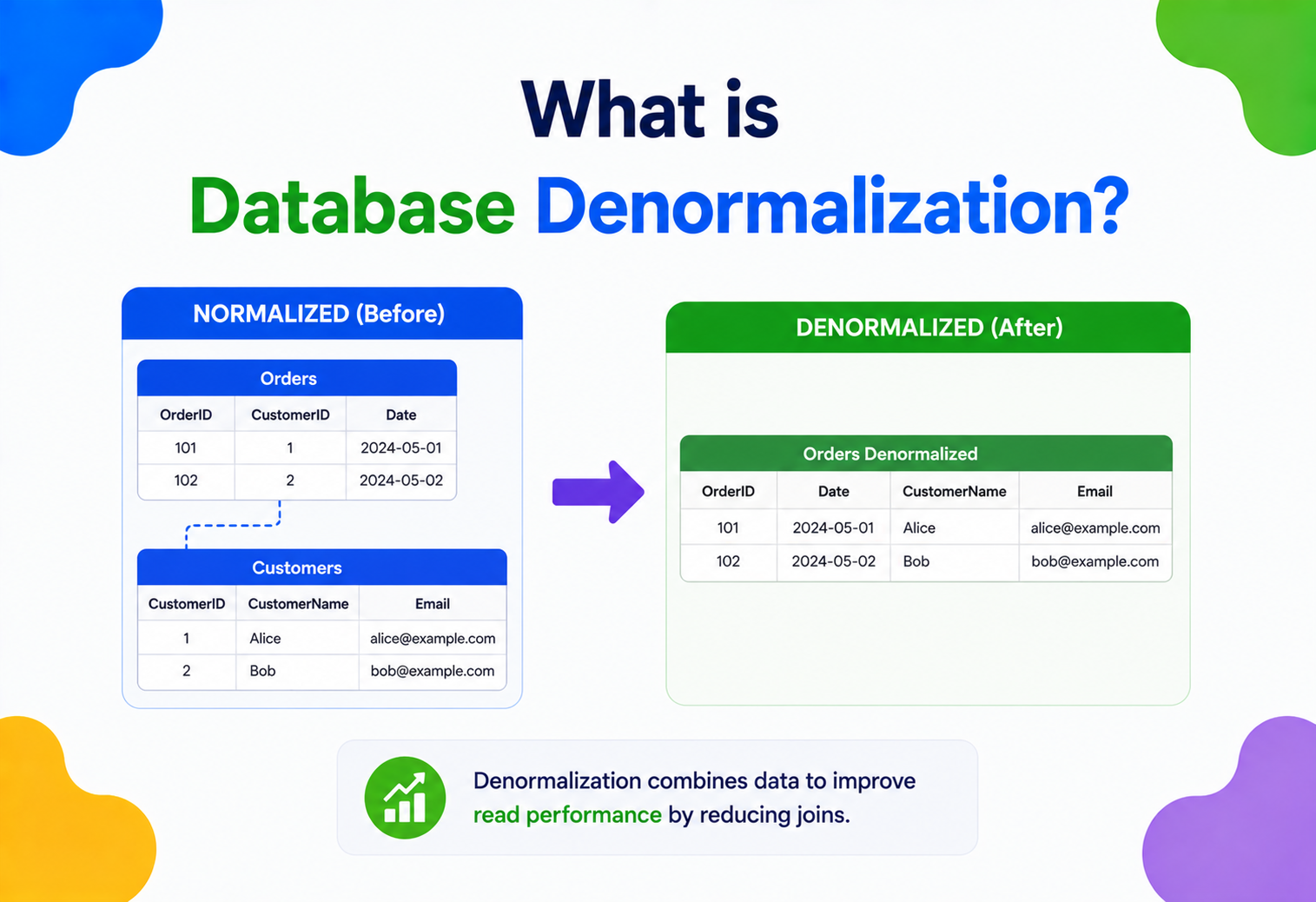
- Duplicating columns — copying a customer’s name directly into the orders table, so you do not need a join to display it.
- Pre‑joining tables — creating one wide table that already contains the combined result of what used to be two or three tables.
- Storing computed / aggregated values — keeping a
total_orderscounter on the customer row instead of runningCOUNT(*)over the orders table every time. - Materialised views — letting the database itself maintain a pre‑computed, join‑free snapshot that refreshes on a schedule or on write.
- Embedding related data — in document databases like MongoDB, nesting related records (like order items) directly inside the parent document instead of a separate collection.
Instagram stores a denormalised like_count directly on each post record. Every time you tap the heart icon, that counter is updated. Without this, showing “12,482 likes” on a popular post would require counting millions of individual “like” rows on every single page view — far too slow at Instagram’s scale.
Architecture & Components
Let us look at the shape of the two designs side‑by‑side. This models a blogging platform with Authors, Posts, and Comments — first the tidy normalised schema, then the wide denormalised read table you would actually query on the hot path.
author_id, post_id); no data is duplicatedTo show a single blog post with the author’s name and comment count, this normalised design needs a join across all three tables. Now compare that to a denormalised version of the POSTS table, built for a fast “reading” experience:
| Column | Purpose |
|---|---|
post_id | Primary key |
title, body | Post content |
author_name | Copied from Authors table — avoids a join to show “by Asha Verma” |
comment_count | Pre‑computed number — avoids counting Comments rows on every view |
latest_comment_snippet | Copied text from the newest comment — avoids a second query entirely |
Now a single row read from one table gives the application everything it needs to render the page. No joins, no counting, no second query. That is the architectural essence of denormalisation: collapse many tables’ worth of data into fewer, wider rows, tuned around how the data will actually be read.
Components involved in a denormalised system
- Source‑of‑truth tables — the original, normalised tables that remain the authoritative record.
- Denormalised read tables / views — the duplicated, wide, read‑optimised copies.
- Synchronisation mechanism — the code, trigger, or pipeline that keeps the copies updated when the source changes (application code, database triggers, message queues, or change‑data‑capture tools like Debezium).
- Consistency window — the (hopefully short) delay between a source update and the denormalised copy catching up, if updates are not perfectly synchronous.
Internal Working
What the database engine is actually doing when you join versus when you read a single denormalised row — and how the picture changes on the write side.
Why joins cost what they cost
When you run a query like SELECT * FROM orders JOIN customers ON orders.customer_id = customers.id, the database engine has to physically locate matching rows across two separate data structures on disk or in memory. It typically uses one of these strategies internally:
- Nested loop join — for each row in table A, scan table B for a match. Simple, but can be slow if tables are large and unindexed (roughly O(n×m) in the worst case).
- Hash join — build an in‑memory hash table of the smaller table’s join column, then scan the larger table and look up matches in O(1) average time per row. Fast, but uses memory.
- Merge join — if both tables are already sorted on the join column, walk through both in lockstep, like zipping two sorted decks of cards together.
Even the fastest join strategy involves more CPU cycles, more memory pressure, and often more disk I/O than reading a single row that already contains everything you need. An index can make a join fast, but it cannot make it free — you are still doing extra work at query time that denormalisation does once, in advance, at write time.
A join is like a substitute teacher who does not know any students by face. To grade an assignment, they must cross‑reference a seating chart and an attendance sheet every single time. A denormalised system is like the assignment paper already having the student’s name pre‑printed on it — no cross‑referencing needed. It took a little extra effort to print the names in advance, but grading is instant afterward.
How denormalised reads work internally
When you read from a denormalised table, the engine performs a much simpler operation: locate the row (usually via a primary key or index lookup — O(log n) with a B‑tree index, or O(1) with a hash index) and return all its columns. No second table needs to be touched. This is why denormalised reads are often 2×–100× faster in real workloads, depending on join complexity and data size.
The data structures behind fast lookups
Whether you normalise or denormalise, the database’s underlying indexing structures decide how fast any given lookup will be. Two structures come up constantly:
- B‑tree index — a balanced tree structure that keeps data sorted and allows searches, insertions, and deletions in roughly O(log n) time. Most relational databases (PostgreSQL, MySQL, SQL Server) use B‑tree indexes by default for primary keys and most secondary indexes. Think of it like a well‑organised phone book: you do not read every name, you jump to roughly the right page and narrow down from there.
- Hash index — maps a key directly to a memory or disk location using a hash function, giving close to O(1) average lookup time for exact‑match queries. Great for “find this exact row,” not useful for range queries like “find everything between March and June.” Systems like Redis and DynamoDB lean heavily on hashing.
Here is the important connection to denormalisation: a well‑indexed join can still be reasonably fast — indexes are not a consolation prize, they are essential regardless of your schema shape. But even a perfectly indexed join does strictly more work than a single indexed lookup on a denormalised row, because the database engine still has to traverse two separate index structures and combine the results, rather than one. Denormalisation does not replace the need for indexes; it reduces the number of index traversals a single logical read requires.
How writes work internally when data is denormalised
The trade‑off shows up on the write side. If a customer changes their name, and that name is duplicated across 50,000 order rows, the write is no longer a single‑row update — it becomes a fan‑out update touching many rows (or triggering an asynchronous background job to update them). Internally, this can be implemented as:
- Synchronous multi‑row update — the application or a database trigger updates all duplicated copies in the same transaction. Strongly consistent, but slower writes.
- Asynchronous propagation — the write to the source table succeeds immediately, and a background process (queue consumer, change‑data‑capture stream) updates the denormalised copies afterward. Fast writes, but there is a brief window where data is inconsistent — this is called eventual consistency.
Data Flow & Lifecycle
Following one piece of data from creation to read — and seeing why the same duplication is sometimes a performance hack and sometimes a business requirement.
Let us trace the full life of a single fact — a product’s price — through a denormalised e‑commerce system.
- Write: an admin updates a product’s price in the normalised
productstable (the single source of truth). - Propagate: a trigger, application‑level write, or event stream notices the change and updates the price copy stored inside any unshipped order line items, product search index, and homepage “featured deals” cache.
- Read: a shopper loads the homepage. The server queries the pre‑built, denormalised “featured deals” table — one fast read, no joins across products, inventory, and pricing tables.
- Expiry / Refresh: cached or materialised denormalised data is refreshed on a schedule (e.g., every 60 seconds) or invalidated immediately on write, depending on how fresh it needs to be.
- Audit: the normalised source table remains the authority for historical correctness — for example, an already‑placed order should usually keep the price at the time of purchase, which is actually a case where “duplicating” the price into the order row is not just a performance hack but the correct business behaviour.
Not all duplication is “for speed.” Sometimes duplicating data is the only correct way to model reality. An order’s price_at_purchase must stay frozen even if the product’s price later changes — copying it is not a performance optimisation here, it is a business requirement. Recognising this distinction is a mark of a senior engineer.
Read‑path vs. write‑path comparison
Normalised design
- Write 1 table, fast, atomic
- Read N joins, slower and heavier on CPU / I/O
- Cost is paid on the read path — every single page view
Denormalised design
- Write N tables / copies to keep in sync, slower
- Read 1 table, single indexed lookup, very fast
- Cost is paid on the write path — usually much less frequent
Fig 6.1 — the trade‑off in one picture: normalisation pushes cost onto reads; denormalisation pushes cost onto writes. You are always choosing which side pays.
Advantages, Disadvantages & Trade‑offs
Weighing it honestly — there is real upside, and real cost, and neither disappears just because you follow best practices.
Advantages
| Benefit | Why it happens |
|---|---|
| Speed Faster reads | No joins needed; data already lives together. |
| Speed Fewer round trips | One query replaces several, reducing network and lock overhead. |
| Simplicity Simpler read queries | Application code does not need complex SQL joins or ORM eager‑loading logic. |
| Scalability Easier horizontal scaling | Self‑contained rows/documents are easier to shard and cache without cross‑shard joins. |
| Analytics Better reporting performance | Pre‑aggregated tables make dashboards and analytics near‑instant. |
Disadvantages
| Cost | Why it happens |
|---|---|
| Consistency risk Data can drift | If a sync step fails or is delayed, duplicated copies can disagree. |
| Storage Uses more space | The same fact exists in multiple places. |
| Write complexity Slower, harder writes | One logical update may require updating many rows or triggering async jobs. |
| Maintenance More code to maintain | Sync logic, triggers, and reconciliation jobs are extra systems that can break. |
| Bugs Harder to debug | “Why does the UI show different values in two places?” becomes a real, recurring question. |
The trade‑off, summarised
Every denormalisation decision is really a bet: “I am confident this data is read far more often than it is written, and I am willing to add engineering complexity to make those reads fast.” If that bet is wrong — if the data is written just as often as it is read, or consistency matters more than speed (like account balances) — denormalisation usually makes the system worse, not better.
Denormalise data that is read far more often than it changes, and where a brief delay in consistency is tolerable. Never denormalise your one true source of financial balances, inventory counts used for allocation, or anything where two slightly different values could cause real‑world harm (double‑selling the last item in stock, for example) — unless you pair it with very careful synchronous updates or reconciliation.
Performance & Scalability
Making the trade‑off pay off at scale — and understanding why the same denormalised row is usually the difference between graceful growth and a service that folds under load.
Read amplification vs. write amplification
Two useful terms:
- Read amplification — the number of extra operations (joins, lookups) needed to answer one logical read. Normalisation tends to increase this.
- Write amplification — the number of extra operations needed to complete one logical write. Denormalisation tends to increase this.
A well‑designed denormalised system deliberately shifts amplification from the read path (which usually has far higher volume — a product page might be viewed 10,000 times for every 1 time its price changes) to the write path (which is comparatively rare). This is a classic engineering trade: optimise for the hot path.
Sharding and partitioning
When a database grows too large for one server, it is split across multiple servers — this is called partitioning or sharding. Joins across shards (cross‑shard joins) are notoriously expensive or even unsupported in many distributed databases, because data has to travel across the network between machines. Denormalisation sidesteps this entirely: if all the data a query needs lives in one row on one shard, there is no cross‑network join at all.
Caching layers
Denormalisation and caching solve a similar problem (slow reads) at different layers. A cache (like Redis) stores computed results temporarily in memory; a denormalised table stores them durably on disk. Many production systems use both: a denormalised table as the “warm” source, and an in‑memory cache in front of it for the very hottest data.
Big‑O intuition
Without indexes, a naive join is roughly O(n × m) — every row in one table potentially checked against every row in the other. With good indexes, this typically improves to about O(n log m). A denormalised single‑row lookup by primary key is close to O(1) (hash index) or O(log n) (B‑tree index). At small n and m, the difference is invisible. At the scale of hundreds of millions of rows, it is the difference between milliseconds and seconds.
High Availability & Reliability
Keeping duplicated data trustworthy under failure — because a denormalised copy that silently disagrees with the source is worse than no copy at all.
Replication
Replication means keeping copies of the same data on multiple servers, so if one server fails, another can take over. This is a form of intentional duplication too — closely related in spirit to denormalisation, but for fault tolerance rather than query speed. Many systems combine both: a normalised primary database, replicated to several read replicas, which in turn feed denormalised, purpose‑built read tables.
CAP theorem, in plain terms
The CAP theorem says that a distributed system cannot simultaneously guarantee all three of: Consistency (everyone sees the same data at the same time), Availability (every request gets a response), and Partition tolerance (the system keeps working even if network links between servers fail). Since network partitions are unavoidable in real distributed systems, you are really choosing between consistency and availability when a partition happens.
Denormalised, asynchronously‑updated data is a practical embrace of the “Availability over Consistency” side of that trade‑off: you accept that a duplicated copy might briefly be stale (an AP choice) in exchange for the system staying fast and responsive even under stress.
Imagine several branches of the same library, each keeping its own copy of the card catalogue. If a phone line between two branches goes down, each branch can still serve customers using its local (possibly slightly outdated) catalogue copy, rather than freezing until the phone line is fixed. That is choosing availability over perfect real‑time consistency.
Consistency models relevant to denormalisation
- Strong consistency — every read sees the latest write immediately. Usually requires synchronous updates across all copies — safer, but slower and less available under failure.
- Eventual consistency — copies converge to the same value eventually, given no new writes. Common with asynchronous denormalisation pipelines. Fast and resilient, but temporarily “wrong.”
- Read‑your‑writes consistency — a middle ground: the user who made a change always sees their own change immediately, even if other users see it slightly later.
Consensus and coordinated updates
When a denormalised value must be updated consistently across multiple independent nodes at the same time — for example, a distributed cache cluster that all needs to agree on a new price simultaneously — distributed systems sometimes reach for consensus algorithms like Raft or Paxos. These algorithms let a group of machines agree on a single value even if some of them fail or messages get delayed or lost, by requiring a majority (“quorum”) of nodes to agree before a value is considered committed. This matters for denormalisation because propagating a change to many replicas is fundamentally a coordination problem: consensus protocols are one rigorous way to make sure that coordination does not silently fail and leave replicas disagreeing forever.
Most everyday denormalisation does not need full consensus machinery — a message queue with retries and a reconciliation job is often good enough. But it is worth recognising that “keep several copies of the same fact in agreement, even under failure” is the same underlying problem that consensus algorithms exist to solve, just at a different scale and with different tolerance for delay.
Concurrency concerns
Denormalised counters and aggregates (like a like count or an inventory total) are especially exposed to race conditions — bugs that happen when two operations run at nearly the same time and interfere with each other. If two requests both read a counter’s current value, each add one, and then both write their result back, one of the increments can be silently lost, because the second write overwrites the first without knowing about it. The fix, shown later in the Java examples, is to perform the increment as a single atomic database operation (like UPDATE ... SET count = count + 1) rather than reading a value into application code, changing it, and writing it back in separate steps.
Failure recovery and reconciliation
Because denormalised copies can drift, production systems typically run reconciliation jobs — batch processes that periodically compare the source of truth to the denormalised copies and repair any mismatches. This is a critical, often‑overlooked piece of real denormalised architectures: you need a safety net for when the sync mechanism inevitably fails (a queue message gets dropped, a worker crashes mid‑update, a network blip occurs).
Security
The often‑missed risk of copied data — every duplicated column is another place a sensitive value has to be protected, deleted, and audited.
Denormalisation has security implications that are easy to overlook:
- Sensitive data spreads. If you copy a customer’s email into ten different tables to speed up reads, you now have ten places that need encryption, access control, and deletion logic — instead of one. This directly affects compliance with privacy laws like GDPR’s “right to be forgotten,” which require deleting a user’s data everywhere, not just in the source table.
- Stale permissions. If a user’s access role is denormalised into many records for speed, revoking their access needs to reach every copy immediately, or they may retain access longer than intended.
- Larger attack surface. More tables / columns holding the same sensitive value means more places a misconfigured permission or SQL injection could expose it.
Maintain a clear, documented map of every place a piece of sensitive data is duplicated to. Automate deletion / anonymisation across all copies as part of any “delete my account” workflow — never assume deleting from the source table is enough.
Monitoring, Logging & Metrics
How you know it is working — and, more importantly, how you know when it is drifting before a customer notices.
A denormalised system needs its own category of monitoring beyond typical database health checks:
- Replication / sync lag — how far behind is the denormalised copy from the source? Usually measured in milliseconds or seconds. Alert if this grows beyond an acceptable threshold.
- Consistency drift rate — the percentage of sampled records where the denormalised copy disagrees with the source, found through periodic reconciliation checks.
- Queue depth / worker throughput — for async propagation pipelines, a growing queue backlog is an early warning sign that sync is falling behind write volume.
- Query latency (p50 / p95 / p99) — the whole point of denormalising is speed, so track percentile latencies before and after to prove the trade‑off actually paid off.
- Failed sync events — log and alert on any failed update to a denormalised copy so it can be retried or reconciled.
Tools like Prometheus (metrics collection), Grafana (dashboards), and distributed tracing systems like Jaeger or OpenTelemetry are commonly used to track sync lag and pipeline health. A simple, high‑value dashboard: “seconds since last successful sync” per denormalised table, with an alert if it exceeds your tolerance (e.g., 30 seconds for a “likes count,” but 0 seconds tolerance for an account balance — which likely should not be denormalised this way at all).
Deployment & Cloud
You rarely have to build denormalisation pipelines entirely from scratch anymore. Cloud providers offer managed building blocks that turn much of this into configuration rather than bespoke code.
- Materialised views — supported natively in PostgreSQL, Oracle, and Snowflake; the database automatically maintains a denormalised, pre‑computed table for you.
- Change Data Capture (CDC) — tools like Debezium, AWS DMS, or Google Cloud Datastream watch a source database’s transaction log and stream every change out, which downstream systems use to keep denormalised copies in sync.
- Managed search / read stores — services like Amazon OpenSearch, Elasticsearch, or DynamoDB are often used as the “read‑optimised, denormalised” side of a system, fed by CDC from a normalised primary database (often called CQRS — Command Query Responsibility Segregation, covered in Design Patterns below).
- Data warehouses — Snowflake, BigQuery, and Redshift are built around wide, denormalised (often “star schema”) tables for analytics, fed by ETL / ELT pipelines from normalised operational databases.
A typical modern pipeline
Databases, Caching & Load Balancing
Where denormalisation fits among its neighbours — indexing, caching, replicas — and how experienced engineers pick between them.
Relational vs. NoSQL, and denormalisation’s role
NoSQL databases (like MongoDB, Cassandra, DynamoDB) often encourage denormalisation as the default modelling approach, rather than an exception. In MongoDB, for example, it is common and idiomatic to embed an order’s line items directly inside the order document, instead of a separate “line items” collection — because these databases are optimised around fast, single‑document reads rather than cross‑collection joins (which are often limited or absent).
| System | Default philosophy |
|---|---|
| PostgreSQL / MySQL (relational) | Normalise by default; denormalise selectively when proven necessary. |
| MongoDB (document store) | Embed / denormalise by default for data accessed together; reference (normalise) only for large or independently‑changing data. |
| Cassandra (wide‑column) | Model tables around specific queries (“query‑first design”), heavily denormalised, often one table per read pattern. |
| Redis (cache / key‑value) | Not a source of truth at all — stores pre‑computed, denormalised results temporarily for speed. |
Choosing between indexing, caching, and denormalisation
These three tools are often confused because they all make reads faster, but they solve different shapes of problem, and experienced engineers reach for them in a fairly predictable order.
| Tool | Best for | What it costs you |
|---|---|---|
| Add an index | A single table is slow to search or filter, but the schema is fine as‑is. | Slightly slower writes; extra storage for the index itself. Usually the cheapest fix — try this first. |
| Add a cache | The same expensive read happens repeatedly and can tolerate being served from memory temporarily. | Cache invalidation complexity; data can be briefly stale; cache can be lost and must be rebuildable. |
| Denormalise | The slowness comes from combining data across multiple tables (joins), not just searching within one. | Write complexity, storage duplication, and an ongoing synchronisation / consistency responsibility. |
In practice, these are not mutually exclusive — a mature system typically layers all three: indexes on the normalised source tables, denormalised tables or materialised views for known‑expensive join patterns, and a cache in front of the very hottest reads of all. The mistake to avoid is reaching for denormalisation as the very first tool, when an index would have solved the problem with far less ongoing complexity.
Load balancing and read replicas
A load balancer distributes incoming requests across multiple servers so no single machine gets overwhelmed. In database architecture, a common pattern is read replicas: copies of the database that only handle read queries, while a single primary handles writes. Denormalised read tables are frequently placed on these replicas, since reads dominate and can be scaled out horizontally, while writes to the source of truth stay centralised and consistent.
Design Patterns & Anti‑patterns
Proven shapes that repeatedly show up in well‑engineered systems — and the classic traps that repeatedly show up in the post‑mortems of ones that broke.
Pattern: Star Schema (data warehousing)
A central “fact” table (e.g., Sales) surrounded by denormalised “dimension” tables (e.g., Product, Store, Date) that are wide and flat rather than further normalised. This is the standard pattern for analytics and business intelligence, because analysts run big aggregate queries (total sales by region by month) where join‑heavy normalised schemas would be painfully slow.
Pattern: CQRS (Command Query Responsibility Segregation)
Separate the model used for writes (“commands”) from the model used for reads (“queries”). Writes go to a normalised store optimised for correctness; reads are served from one or more denormalised projections optimised for speed, kept in sync via events. This is common in large e‑commerce and social platforms.
Pattern: Event Sourcing + Projections
Instead of storing current state directly, the system stores an append‑only log of every event that ever happened (e.g., “ItemAddedToCart”, “PriceChanged”). Denormalised “read models” (projections) are rebuilt or updated from this event log — giving you both a perfect audit trail and fast, purpose‑built read tables.
Pattern: Precomputed Aggregates / Rollups
Storing running totals, counts, or summaries (like total_likes, monthly_revenue) instead of recalculating them from raw rows on every read. Usually updated incrementally on write (e.g., UPDATE posts SET like_count = like_count + 1) rather than recomputed from scratch.
Anti‑pattern: Denormalising too early
Adding duplication before you have evidence (real traffic patterns, real slow queries) that you need it. This adds complexity for a problem that may never materialise. The professional default is: normalise first, measure, then denormalise the specific hot paths that actually need it.
Anti‑pattern: No synchronisation strategy
Duplicating data without a clear, tested, monitored process for keeping copies updated. This is the single most common cause of “our numbers do not match” bugs in production systems.
Anti‑pattern: Denormalising frequently‑changing data
Copying a value that changes every few seconds (like a live stock price) into many places creates a constant, expensive fan‑out of updates — often worse than the join it was meant to avoid. Denormalisation pays off best for data that is read far more often than it is written.
Anti‑pattern: Treating denormalised copies as a second source of truth
If application code ever writes directly to a denormalised copy without also updating (or deriving from) the source of truth, you now have two competing authorities for the same fact — a recipe for silent, hard‑to‑trace bugs.
Best Practices & Common Mistakes
What experienced teams actually do — and a set of Java examples showing the difference between a joined read, a denormalised read, an atomic counter update, and a transactionally‑consistent fan‑out.
Best practices
- Normalise first, denormalise with evidence. Start clean. Use real slow‑query logs or load testing to identify actual hot paths before duplicating anything.
- Keep one clear source of truth per fact. Denormalised copies should always be derived from, never independently edited apart from, the source.
- Automate synchronisation — never rely on developers remembering. Use database triggers, application‑layer write wrappers, or event‑driven pipelines, not “please remember to update both tables” tribal knowledge.
- Monitor for drift. Build reconciliation jobs and alerting so silent inconsistency gets caught, not discovered by an angry customer.
- Document every duplicated field. Maintain a simple registry: what is duplicated, where, why, and how it is kept in sync.
- Prefer database‑native tools where possible. Materialised views, generated columns, and triggers are often more reliable than hand‑rolled application logic.
- Version your denormalised schema deliberately. Changing a denormalised structure often requires a backfill migration across potentially huge tables — plan for it.
Common mistakes
- Denormalising the entire database “just in case,” instead of specific proven bottlenecks.
- Forgetting to update all duplicate locations when writing new features — usually because the duplication was not documented.
- Using denormalisation to paper over a missing index, when a well‑placed index would have solved the performance problem more simply.
- Denormalising financial or safety‑critical data without strong consistency guarantees.
- No plan for schema evolution — realising a year later that fixing a denormalised field requires rewriting billions of rows.
A worked Java example
Below is a simplified example showing the difference between a normalised read (requiring a join) and a denormalised read (a single query), followed by a safe way to keep a denormalised counter updated using a single atomic SQL statement rather than “read, modify in Java, write back” — which would be vulnerable to race conditions under concurrent requests.
public Order getOrderNormalized(Connection conn, long orderId) throws SQLException {
    String sql = """
        SELECT o.id, o.product, o.price, c.name AS customer_name
        FROM orders o
        JOIN customers c ON o.customer_id = c.id
        WHERE o.id = ?
        """;
    try (PreparedStatement ps = conn.prepareStatement(sql)) {
        ps.setLong(1, orderId);
        try (ResultSet rs = ps.executeQuery()) {
            if (rs.next()) {
                return new Order(
                    rs.getLong("id"),
                    rs.getString("product"),
                    rs.getBigDecimal("price"),
                    rs.getString("customer_name")
                );
            }
        }
    }
    return null;
}public Order getOrderDenormalized(Connection conn, long orderId) throws SQLException {
// customer_name is already stored on the orders row itself
String sql = "SELECT id, product, price, customer_name FROM orders_denormalized WHERE id = ?";
try (PreparedStatement ps = conn.prepareStatement(sql)) {
ps.setLong(1, orderId);
try (ResultSet rs = ps.executeQuery()) {
if (rs.next()) {
return new Order(
rs.getLong("id"),
rs.getString("product"),
rs.getBigDecimal("price"),
rs.getString("customer_name")
);
}
}
}
return null;
}public void incrementLikeCount(Connection conn, long postId) throws SQLException {
// Atomic, single-statement increment done inside the database itself.
// Never do "SELECT count, then count+1 in Java, then UPDATE" —
// two concurrent requests could both read the same starting value
// and one increment would be silently lost.
String sql = "UPDATE posts SET like_count = like_count + 1 WHERE id = ?";
try (PreparedStatement ps = conn.prepareStatement(sql)) {
ps.setLong(1, postId);
ps.executeUpdate();
}
}public void updateCustomerName(Connection conn, long customerId, String newName) throws SQLException {
conn.setAutoCommit(false);
try {
// 1. Update the source of truth
try (PreparedStatement ps = conn.prepareStatement(
"UPDATE customers SET name = ? WHERE id = ?")) {
ps.setString(1, newName);
ps.setLong(2, customerId);
ps.executeUpdate();
}
// 2. Propagate to the denormalized copy in the same transaction
// (synchronous approach — simple, strongly consistent, but
// slower if a customer has many orders; an async queue-based
// approach is often preferred at very large scale)
try (PreparedStatement ps = conn.prepareStatement(
"UPDATE orders_denormalized SET customer_name = ? WHERE customer_id = ?")) {
ps.setString(1, newName);
ps.setLong(2, customerId);
ps.executeUpdate();
}
conn.commit();
} catch (SQLException e) {
conn.rollback();
throw e;
} finally {
conn.setAutoCommit(true);
}
}Notice the pattern in the last example: both updates happen inside one transaction, so either both succeed or both roll back together — the denormalised copy can never “half update” and drift from the source.
Real‑World & Industry Examples
How the giants actually use this — and, just as importantly, one contrasting example of a system that deliberately does not, to show that denormalisation is a choice, not a universal rule.
Precomputed homepage rows
Netflix serves personalised homepage rows (“Continue Watching,” “Because You Watched…”) to over 250 million member profiles. Computing these recommendations live from normalised viewing‑history tables for every single homepage load would be far too slow. Instead, Netflix precomputes and denormalises recommendation results into fast‑access stores (built on systems like Cassandra and EVCache), refreshed by large offline and near‑real‑time pipelines, so the homepage loads in a fraction of a second.
Pre‑assembled product pages
Amazon’s product pages combine data that, in a normalised world, would live across inventory, pricing, reviews, and seller tables. Amazon builds denormalised, pre‑assembled product‑page data ahead of time, so a single page load does not have to assemble it live from many microservices and tables on every request — critical at Amazon’s scale of billions of page views.
Trip matching in milliseconds
Uber’s trip‑matching and pricing systems need to answer “what is near me right now” in milliseconds. Rather than joining live driver‑location tables with trip and pricing tables on every request, Uber maintains denormalised, frequently‑refreshed spatial indexes and pricing snapshots optimised purely for fast lookups, with the authoritative trip and billing data reconciled separately in normalised backend systems.
Counts on every post
As mentioned earlier, like counts, follower counts, and comment previews shown on every post are denormalised, precomputed values — not counted live from billions of underlying rows on every scroll. Meta’s infrastructure (built on systems like TAO, a graph‑caching layer over MySQL) is specifically designed around this pattern: cache and denormalise aggressively for reads, propagate writes asynchronously.
A contrasting example
Core account balance and ledger systems at banks are deliberately kept close to normalised and strongly consistent — because an inconsistent, briefly‑stale balance could mean double‑spending money or an incorrect overdraft decision. This is a useful contrast: it shows denormalisation is a deliberate choice made where it is safe, not a rule applied everywhere.
Read‑heavy hot paths win
Every one of the big‑scale examples above shares the same shape: a tiny handful of write events per second are answered by orders of magnitude more read events per second. Deliberate duplication is how that ratio gets served without the read path collapsing.
FAQ, Summary & Key Takeaways
Wrapping it up — the questions that come up over and over, the summary in a paragraph, a quick‑reference glossary, and the ideas worth carrying into every future design conversation.
Frequently asked questions
Is denormalisation the same as “bad database design”?
No. Bad design is accidental, undocumented duplication with no synchronisation plan. Denormalisation is deliberate, measured duplication with a clear reason, a clear source of truth, and a plan for keeping copies in sync.
Should I normalise or denormalise when starting a new project?
Normalise first. It is the safer default — easier to keep correct, and you can always denormalise specific hot paths later once you have real evidence (actual slow queries, actual traffic patterns) that you need to.
Does NoSQL mean I do not need to think about normalisation at all?
You still need to think about it — you are just making the trade‑off earlier and more explicitly. Document‑oriented databases push you toward denormalised (“embedded”) designs by default, but you still choose what to embed versus reference based on how data is accessed and how often it changes.
What is the difference between denormalisation and caching?
A cache is typically a temporary, in‑memory copy that can be safely lost and rebuilt (like Redis). A denormalised table is typically a durable, disk‑stored part of your permanent schema. In practice, teams often use both together: a denormalised table as a durable “warm” layer, with a cache in front of it for the hottest reads.
How do I know when it is time to denormalise?
Look for: slow, join‑heavy queries showing up repeatedly in your slow‑query logs; a read‑to‑write ratio that is heavily skewed toward reads for that data; and a clear, specific user‑facing page or feature that is suffering because of it. If you cannot point to a specific, measured problem, it is usually too early.
Can denormalisation actually make a system slower?
Yes, in two common situations. First, if the duplicated data changes very frequently, the overhead of keeping every copy updated can exceed the cost of the joins it was meant to avoid. Second, if a denormalised table becomes extremely wide (many duplicated columns), scanning or writing whole rows can become slower than working with smaller, focused normalised tables, especially for row‑based storage engines. Denormalisation is a targeted tool, not a universal speed boost.
Do I need special tools to denormalise, or can I do it by hand?
You can absolutely do it by hand — with application code, careful transactions, and discipline. Many teams start this way. As the number of duplicated fields grows, though, most teams migrate toward database‑native tools (materialised views, generated columns, triggers) or event‑driven pipelines (change data capture, message queues), because hand‑written synchronisation logic tends to accumulate bugs and blind spots as a codebase grows and more engineers touch it over time.
Is denormalisation only relevant for huge companies like Netflix or Amazon?
No — the principle scales down. Even a small application with a few thousand users can benefit from denormalising a single expensive dashboard query or a report that used to take several seconds to generate. The difference at large scale is mostly about the sophistication of the synchronisation tooling required, not whether the underlying idea applies.
Summary
Normalisation organises data so every fact lives in exactly one place, keeping databases small, consistent, and safe to update — the right default for most systems. But that cleanliness has a cost: reading combined data requires joins, which get expensive as data and traffic grow. Denormalisation is the deliberate, engineered decision to duplicate or pre‑combine data so reads become fast single‑table lookups, accepting the cost of more complex, carefully synchronised writes in exchange.
It shows up everywhere in production systems at scale — from a simple like_count column on a social media post, to entire data warehouses built around denormalised star schemas, to industry‑standard patterns like CQRS and materialised views. The engineers who use it well share a common discipline: they normalise by default, measure before optimising, keep one clear source of truth, automate synchronisation instead of trusting memory, and monitor relentlessly for drift.
Quick‑reference glossary
| Term | Plain‑English meaning |
|---|---|
| Normalisation | Splitting data so every fact is stored exactly once, linked by small ID pointers. |
| Denormalisation | Deliberately copying or pre‑combining data so it can be read without extra lookups. |
| Join | Combining rows from two or more tables based on a matching column, at query time. |
| Redundancy | The same fact stored in more than one place. |
| Anomaly (update/insert/delete) | A bug caused by duplicated data becoming inconsistent or unrepresentable. |
| Materialised view | A saved, pre‑computed query result that the database maintains like a real table. |
| Eventual consistency | Copies of data will match eventually, but might briefly disagree right after a write. |
| Read / write amplification | Extra work a single logical read or write triggers under the hood. |
| Sharding / partitioning | Splitting one large dataset across multiple servers to scale beyond one machine’s limits. |
| CQRS | Using a different data model for writing data than the one used for reading it. |
| Star schema | A denormalised warehouse layout: one fact table surrounded by wide, flat dimension tables. |
Key takeaways
- Normalisation avoids repeating data; denormalisation repeats it on purpose, for speed.
- The classic trade‑off: normalisation pushes cost onto reads (via joins); denormalisation pushes cost onto writes (via synchronisation).
- Denormalise data that is read far more often than it changes, and where brief staleness is acceptable.
- Never denormalise without a clear source of truth and an automated, monitored synchronisation strategy.
- Modern cloud tools — materialised views, change data capture, event streams — make safe denormalisation far easier than hand‑rolled application code.
- Real production giants (Netflix, Amazon, Uber, Meta) rely on denormalisation extensively for anything read at massive scale.
- The professional default is: normalise first, measure, then denormalise deliberately where evidence justifies it.