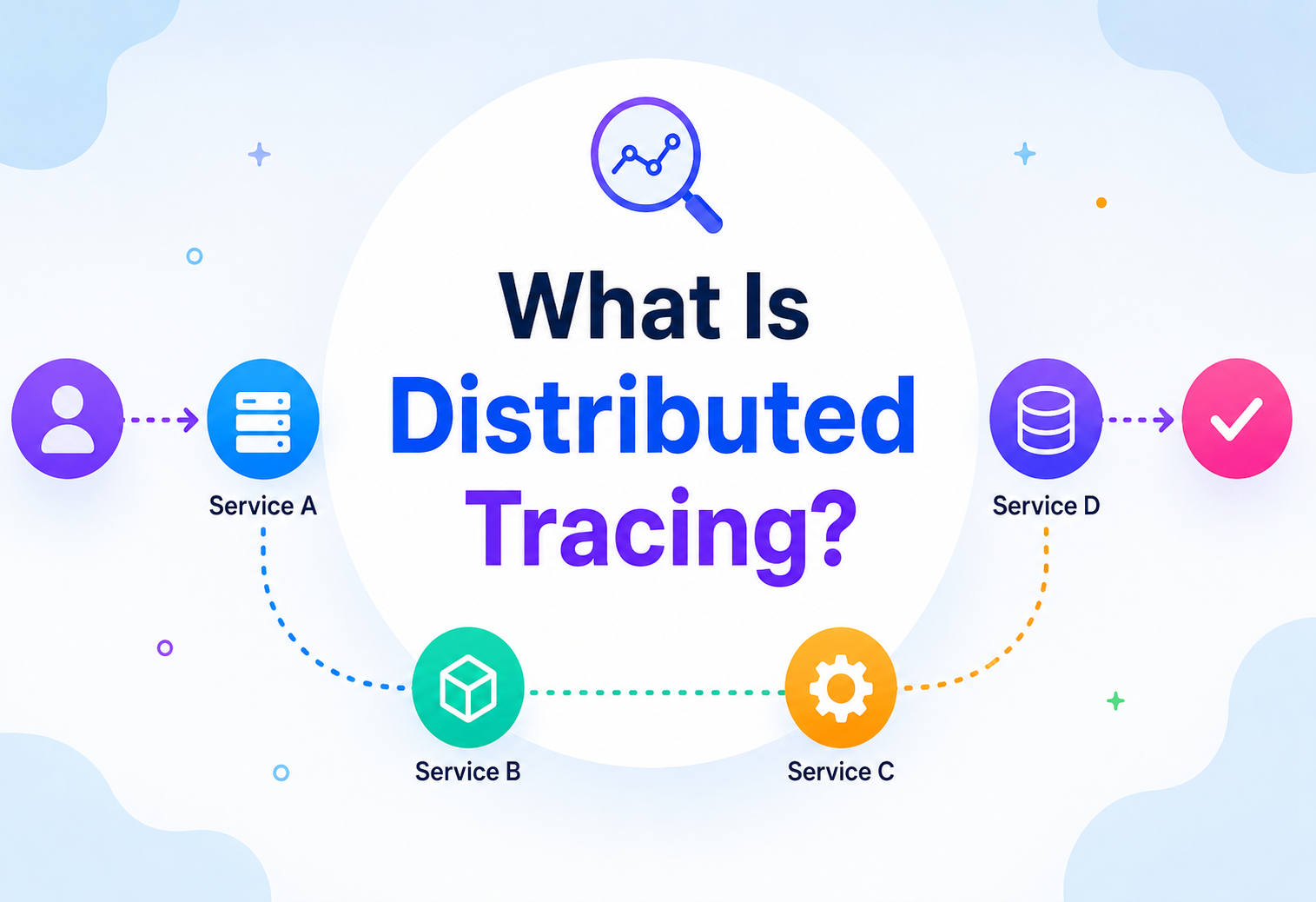
What Is Distributed Tracing?
A beginner-friendly, deeply technical walkthrough of how modern systems follow a single request as it hops through dozens of microservices — simple enough for a curious ten-year-old, rigorous enough for a production engineer.
Introduction & History
Before any theory, one everyday story to make the whole idea click in a single image.
Imagine you order a pizza online. You tap “Order,” and a few seconds later you see “Order Confirmed.” That single tap actually triggers a whole chain of invisible work: checking your payment, reserving ingredients at the store, notifying the kitchen, assigning a delivery driver, and sending you a confirmation text. If your order is late, how would anyone figure out which step went wrong? Was it the payment system? The kitchen? The delivery app?
Distributed tracing is the technique software engineers use to answer exactly this kind of question, but for computer systems instead of pizza orders. It records the journey of a single request as it hops from one service to another, so that when something is slow or broken, engineers can see the entire path and pinpoint the exact weak link.
Think of a relay race with 10 runners, except each runner is in a different stadium, in a different city. Distributed tracing is like giving the baton a tiny GPS tracker and a stopwatch. Even though no single person can watch all 10 stadiums at once, the tracker gives you a complete replay afterward: who ran when, how long each leg took, and exactly where the baton got stuck.
1.1 · A short history
In the early days of software, most applications were “monoliths” — one big program running on one or a few servers. If something broke, you opened one log file and read it top to bottom. Debugging was tedious but straightforward because everything happened in one place.
Around the mid-2000s, companies like Google, Amazon, and eBay started splitting their giant applications into many small, independently deployed services — what we now call microservices. This solved a lot of problems (teams could move faster, scale independently, and use different technologies), but it created a new nightmare: a single user request might now touch 20, 50, or even hundreds of services. No single log file could show the whole picture anymore.
In 2010, Google published a landmark paper called “Dapper, a Large-Scale Distributed Systems Tracing Infrastructure.” It described how Google tracked requests across its massive internal service fleet using lightweight, sampled tracing. Dapper became the blueprint that almost every tracing system since has borrowed from.
Following Dapper, several open-source tracing systems emerged: Zipkin (built at Twitter, inspired directly by Dapper), Jaeger (built at Uber), and later a standardisation effort that merged two earlier projects — OpenTracing and OpenCensus — into what is now the industry standard: OpenTelemetry (OTel). Today, OpenTelemetry is a Cloud Native Computing Foundation (CNCF) project and is the recommended way to instrument new applications for tracing, metrics, and logs together.
Problem & Motivation
Before we go further, let’s clearly understand why distributed tracing had to be invented. Every good tool exists because of a painful problem it solves.
2.1 · The monolith world (easy debugging)
In a monolithic application, one process handles the entire request. If a user complains “checkout is slow,” an engineer opens the application logs, and everything — database calls, business logic, external API calls — is right there, in order, in one file.
2.2 · The microservices world (hard debugging)
Now picture an e-commerce checkout built as microservices: an API Gateway calls the Order Service, which calls the Inventory Service and the Payment Service in parallel, and the Payment Service calls a third-party bank API. Each of these runs as a separate process, often on separate machines, sometimes in separate data centres.
If checkout is slow, which log file do you open? Each service writes its own logs, with its own timestamps, and no shared identifier connecting them. You’d have to manually guess timestamps and stitch together six or seven log files by hand. At 3 AM, during an outage, with customers complaining — this is a nightmare.
When a single logical request is served by many independent services, there is no built-in way to see the “whole story” of that request. Logs are scattered, disconnected, and often stored on different machines entirely.
2.3 · What engineers needed
- A single ID that follows a request everywhere it goes, so all related logs can be grouped together.
- Timing information for every step, so slow steps can be identified.
- A visual map of which service called which, and in what order (sequential vs. parallel).
- Low overhead — the tracking itself must not slow down the very system it’s monitoring.
Distributed tracing was built to satisfy exactly these four needs. It is one of the “three pillars of observability” — alongside logs and metrics — and it is specifically the pillar that shows the path and timing of a single request across service boundaries.
Core Concepts
Before diagrams and code, we need a shared vocabulary. Each term below is explained from scratch.
3.1 · Trace
- What
- A trace represents the complete journey of one single request through your entire system, from the moment it enters (say, a user clicking “Buy Now”) to the moment the final response is sent back.
- Why
- Without a trace, you only see fragments — individual service logs — not the full journey.
- Where
- Every time you debug “why was this one request slow,” you look at its trace.
- Analogy
- A trace is like the full flight itinerary of a passenger travelling from Delhi to New York with two layovers. It’s not just one flight — it’s the entire journey, all connected flights included.
3.2 · Span
- What
- A span is one unit of work within a trace — for example, “Order Service calls Inventory Service” is one span. A trace is made up of many spans, and spans can contain other spans (parent-child relationships).
- Why
- A trace alone is too coarse; you need to break it into individual steps to know exactly which step was slow.
- Simple
- If a coffee shop order has three steps — take order, make coffee, hand it over — each step is a span, and the whole order is the trace.
- Software
- A span typically records: a name (e.g.
GET /inventory/check), a start time, a duration, a status (success/error), and key-value tags (e.g.http.status_code=200).
3.3 · Trace ID and Span ID
- What
- A Trace ID is a unique identifier (usually a 128-bit random number) assigned to a request the moment it enters the system. Every span belonging to that request carries the same Trace ID. Each individual span also has its own unique Span ID, plus a reference to its Parent Span ID (except the very first span, called the root span).
- Analogy
- Think of the Trace ID as a tracking number on a courier package (like “AWB1234567”) — it stays the same no matter how many trucks, warehouses, or planes the package passes through. The Span ID is like a stamp at each individual checkpoint (“scanned at Warehouse B, 2:14 PM”).
3.4 · Context propagation
- What
- The mechanism by which the Trace ID and current Span ID are passed from one service to the next, typically inside HTTP headers or message queue metadata.
- Why
- Without propagation, each service would generate its own unrelated Trace ID, and you could never connect the dots.
- Where
- Every outgoing HTTP call, gRPC call, or message published to a queue carries these headers automatically once tracing is set up.
3.5 · The W3C Trace Context standard
Early tracing tools each invented their own header formats (Zipkin used X-B3-TraceId, for example). This caused compatibility headaches. Today, the W3C (World Wide Web Consortium) has standardised a single header format called traceparent, which looks like this:
traceparent: 00-4bf92f3577b34da6a3ce929d0e0e4736-00f067aa0ba902b7-01
             |  |------------trace-id-----------| |--span-id----|  |
           version                                              flags
Almost all modern tracing tools, including OpenTelemetry, support this standard by default, which means services written in different languages by different teams can still participate in the same trace.
3.6 · Sampling
- What
- Recording every single trace for every single request, at very high traffic (say, a million requests per second), would be extremely expensive in storage and processing. Sampling means only keeping a percentage of traces — for example, 1 in every 100 requests, or always keeping traces that had an error.
- Why
- To balance the cost of storing tracing data against the usefulness of having enough data to spot problems.
Common strategies:
- Head-based sampling: The decision to keep or drop a trace is made at the very start (the “head”) of the request, before any spans are even created. Fast and cheap, but risks dropping traces that would later turn out to be interesting (e.g. an error occurring deep inside the call chain).
- Tail-based sampling: The decision is made only after the entire trace is complete (the “tail”), so you can specifically keep all traces with errors or high latency, and randomly sample the rest. More powerful, but requires buffering all spans somewhere until the trace finishes.
3.7 · Instrumentation
- What
- The process of adding tracing code to an application, either manually (writing code that creates spans) or automatically (using an agent or library that intercepts common operations like HTTP calls and database queries without you writing extra code).
- Where
- Almost every popular framework today (Spring Boot, Express.js, Django) has auto-instrumentation libraries available.
3.8 · Span kinds
- What
- Every span is tagged with a “kind” that describes what role it plays in a network interaction.
The five standard kinds in OpenTelemetry are:
- SERVER: A span representing the handling of an incoming request (e.g., a REST endpoint receiving a call).
- CLIENT: A span representing an outgoing call to another service (e.g., making an HTTP request to a downstream API).
- INTERNAL: A span representing work that doesn’t cross a network boundary at all (e.g., an internal calculation or a local function that’s still worth timing).
- PRODUCER: A span representing the act of publishing a message to a queue or event stream.
- CONSUMER: A span representing the act of receiving and processing a message from a queue.
Why it matters: Span kind helps tracing UIs draw more accurate diagrams — for example, correctly pairing a CLIENT span in Service A with the matching SERVER span in Service B, even though they’re technically two separate spans recorded by two separate processes.
3.9 · Baggage
- What
- While trace context (Trace ID, Span ID) is the minimum information needed to connect spans, baggage lets you propagate additional custom key-value data alongside the request — for example, a customer’s subscription tier (“premium” vs “free”) — so that every downstream service can access it without needing to look it up again from a database.
Baggage is added to every single outgoing request header for the lifetime of the trace, so it should be kept small. Overusing baggage for large payloads adds real network overhead to every hop.
3.10 · Summary table of core terms
| Term | One-line meaning | Real-world equivalent |
|---|---|---|
| Trace | Full journey of one request | Entire flight itinerary |
| Span | One step / unit of work | One flight leg |
| Trace ID | Unique ID for the whole journey | Booking reference number |
| Span ID | Unique ID for one step | Individual boarding pass |
| Context propagation | Carrying IDs across service calls | Passing your ticket at each checkpoint |
| Sampling | Deciding which traces to keep | Randomly auditing some shipments, not all |
Architecture & Components
A production-grade distributed tracing system is made up of four major building blocks. Let’s walk through each one.
-
Instrumentation Layer (SDK / Agent)
This lives inside your application code. It creates spans, attaches tags, and injects/extracts trace context from requests. OpenTelemetry provides SDKs for Java, Python, Go, Node.js, .NET, and more, plus auto-instrumentation agents that require zero code changes for many popular frameworks.
-
Collector
Applications don’t usually send trace data directly to long-term storage. Instead, they send it to a nearby lightweight process called a Collector (in OpenTelemetry, this is the OpenTelemetry Collector). The collector receives spans, can batch them, filter them, redact sensitive fields, apply sampling decisions, and then forward them onward.
-
Storage Backend
Trace data is high-volume and write-heavy, so it’s usually stored in databases optimised for this pattern, such as Elasticsearch, Cassandra, or specialised time-series/columnar stores. Cloud vendors offer managed equivalents (AWS X-Ray, Google Cloud Trace, Azure Monitor).
-
Query & Visualisation UI
This is the dashboard engineers actually look at — tools like Jaeger UI, Zipkin UI, or commercial platforms (Datadog APM, Honeycomb, Grafana Tempo + Grafana). These let you search by Trace ID, filter by service or error status, and see a visual “waterfall” chart of spans.
Notice that the application services never talk directly to the storage database. This separation keeps applications simple and lets the observability team change storage backends without touching any application code.
Internal Working
Let’s go one level deeper and see exactly what happens, step by step, when a request flows through two services.
5.1 · Step-by-step walkthrough
- Request arrives at Service A (say, the API Gateway). Since there’s no existing trace context in the incoming request, the tracing library generates a brand-new Trace ID (e.g.
abc123) and creates the root span with a new Span ID (e.g.span-01). - Service A does some work, then needs to call Service B. Before making that HTTP call, the tracing library injects the trace context into the outgoing request headers:
traceparent: 00-abc123-span01-01. - Service B receives the request. Its tracing library extracts the trace context from the incoming headers. It sees Trace ID
abc123already exists, so instead of starting a new trace, it creates a child span (Span IDspan-02) with Parent Span IDspan-01. - Service B does its work (maybe queries a database), records that as another child span, finishes, and returns its response to Service A.
- Service A finishes its root span and marks it complete, then returns the final response to the client.
- In the background (asynchronously, so it never blocks the actual request), both services export their completed spans to the Collector.
- The Collector batches spans and forwards them to storage, where all spans sharing Trace ID
abc123get grouped together into one complete trace.
Exporting spans always happens after the actual business logic response is already on its way back to the user. Tracing should never add noticeable latency to the user-facing request — it works “out of band.”
5.2 · Java example: manual span creation with OpenTelemetry
Below is a minimal example showing how a Java service creates a span manually using the OpenTelemetry SDK. In real projects, most of this is done automatically by auto-instrumentation agents, but seeing it manually helps you understand what’s happening underneath.
import io.opentelemetry.api.trace.Span;
import io.opentelemetry.api.trace.Tracer;
import io.opentelemetry.api.trace.StatusCode;
import io.opentelemetry.context.Scope;

public class InventoryService {

    private final Tracer tracer;

    public InventoryService(Tracer tracer) {
        this.tracer = tracer;
    }

    public boolean checkStock(String productId) {
        // Start a new span; OpenTelemetry automatically links it
        // to the current trace context if one already exists.
        Span span = tracer.spanBuilder("checkStock")
                .setAttribute("product.id", productId)
                .startSpan();

        try (Scope scope = span.makeCurrent()) {
            boolean available = queryDatabase(productId);
            span.setAttribute("stock.available", available);
            return available;
        } catch (Exception e) {
            span.recordException(e);
            span.setStatus(StatusCode.ERROR, "stock check failed");
            throw e;
        } finally {
            span.end(); // Always close the span, even on failure
        }
    }

    private boolean queryDatabase(String productId) {
        // Simulated DB call
        return true;
    }
}
Three things to notice here, explained simply:
tracer.spanBuilder("checkStock").startSpan()— this is like starting a stopwatch and writing down “starting step: checkStock.”span.setAttribute(...)— this attaches useful sticky notes to the span, so later you can search “show me all spans wherestock.available = false.”span.end()in thefinallyblock — this stops the stopwatch, guaranteed to happen whether the method succeeds or throws an error.
5.3 · Java example: propagating context on an outgoing HTTP call
The earlier example showed a span being created. Now let’s see how that span’s context is actually injected into an outgoing HTTP request, so the next service can pick it up.
import io.opentelemetry.api.trace.Span;
import io.opentelemetry.context.Context;
import io.opentelemetry.context.propagation.TextMapSetter;
import io.opentelemetry.api.OpenTelemetry;
import java.net.http.HttpRequest;

public class PaymentClient {

    private final OpenTelemetry otel;

    // Tells OpenTelemetry how to write a header onto our specific
    // HTTP request builder type.
    private static final TextMapSetter<HttpRequest.Builder> SETTER =
        (builder, key, value) -> builder.header(key, value);

    public PaymentClient(OpenTelemetry otel) {
        this.otel = otel;
    }

    public HttpRequest buildChargeRequest(String orderId) {
        HttpRequest.Builder builder = HttpRequest.newBuilder()
                .uri(java.net.URI.create("https://payments.internal/charge"))
                .POST(HttpRequest.BodyPublishers.ofString(orderId));

        // Inject the current trace context (Trace ID + current Span ID)
        // into the outgoing request's headers as "traceparent".
        otel.getPropagators().getTextMapPropagator()
            .inject(Context.current(), builder, SETTER);

        return builder.build();
    }
}
In plain words: inject() looks at “which span is currently active on this thread,” converts its Trace ID and Span ID into the standard traceparent header format, and writes that header onto the outgoing request — exactly like writing a tracking number onto a parcel before handing it to the courier.
Data Flow & Lifecycle
Let’s visualise an entire realistic e-commerce checkout request across five services, and see the resulting trace as a “waterfall” — the same view you’d actually see in a tool like Jaeger.
6.1 · What the resulting trace looks like (waterfall view)
Trace ID: abc123    Total duration: 420ms

[Gateway: POST /checkout] ################################  420ms
  [Order: createOrder]      ##########################      380ms
    [Inventory: checkStock]  #####                            60ms
    [Payment: charge]              #####################     290ms
      [Bank: authorize]                #################     260ms
This kind of chart instantly answers the question “why was checkout slow?” — here, it’s obvious that the Bank authorisation call (260 ms) is the dominant cost, not the Inventory check (60 ms).
6.2 · Lifecycle of a single span
Advantages, Disadvantages & Trade-offs
An honest ledger of what distributed tracing gives you — and what it costs to run responsibly.
PROSAdvantages
- Pinpoints the exact slow or failing service in seconds instead of hours.
- Shows the true shape of a request (sequential vs. parallel calls), which is often surprising even to the engineers who built the system.
- Helps quantify the cost of each dependency, guiding optimisation priorities.
- Makes onboarding new engineers faster — they can literally see how the system behaves instead of reading stale diagrams.
- Essential for meeting Service Level Objectives (SLOs) in complex systems.
CONSDisadvantages & trade-offs
- Adds a small amount of CPU and network overhead to every instrumented call.
- Storage costs can grow quickly at high traffic if sampling isn’t tuned properly.
- Requires discipline: every new service must propagate context correctly, or the trace “breaks” into disconnected fragments.
- Sensitive data can accidentally leak into span attributes if instrumentation isn’t reviewed carefully.
- Initial setup and cultural adoption (getting every team to instrument their service) takes real effort.
Distributed tracing trades a small, constant “tax” on every request (a bit of extra CPU, memory, and network use) for a huge gain in your ability to understand and fix problems quickly. For almost every system with more than a handful of services, this trade is well worth it.
Performance & Scalability
At small scale, tracing every single request is fine. At large scale (think: an app handling 500,000 requests per second), tracing everything would generate more data than the actual application traffic itself. This section covers how tracing systems stay fast and affordable at scale.
8.1 · Sampling strategies in detail
| Strategy | How it decides | Pros | Cons |
|---|---|---|---|
| Fixed-rate (probabilistic) | Keep X% of traces, chosen randomly | Simple, predictable cost | May miss rare but important errors |
| Rate-limiting | Keep at most N traces per second | Protects backend from traffic spikes | Can under-sample during real incidents |
| Tail-based (error/latency aware) | Keep all error traces + slow traces + a sample of normal ones | Never misses the interesting cases | Needs buffering; more collector resources |
| Adaptive sampling | Sampling rate adjusts automatically based on traffic volume | Balances cost and coverage dynamically | More complex to reason about |
8.2 · Reducing overhead
- Asynchronous export: Spans are batched and sent in the background, never blocking the actual request-response cycle.
- Batching: Instead of sending each span individually (expensive, many small network calls), SDKs buffer spans and send them in batches every few seconds.
- Local aggregation at the Collector: The Collector can pre-process data before sending it further, reducing load on the storage backend.
8.3 · Scalability of the storage layer
Trace storage systems typically use a write-optimised database because tracing generates far more writes than reads. Two common patterns:
- Horizontal partitioning (sharding): Trace data is split across many storage nodes, often by Trace ID hash, so no single node becomes a bottleneck.
- Time-based retention: Old traces (say, older than 7 or 30 days) are automatically deleted or moved to cheaper cold storage, since traces are mostly useful for recent debugging, not long-term analytics (that’s what metrics and logs are better suited for).
High Availability & Reliability
A tracing system is a support system — it should never become a reason your actual application goes down. Here’s how reliability is engineered in.
9.1 · Fail open, never fail closed
If the Collector is unreachable, the application should simply drop the trace data and continue serving the real request normally. Tracing must never throw an error that breaks the user-facing request just because the tracing backend is having trouble.
Some early, poorly designed instrumentation made trace export a synchronous, blocking call. If the collector was slow, the whole application became slow too. Modern SDKs use bounded, in-memory queues with a “drop oldest” policy specifically to avoid this trap.
9.2 · Collector high availability
In production, Collectors are typically deployed as a horizontally scaled fleet behind a load balancer, often running as a DaemonSet (one collector per machine, in Kubernetes terms) or as a centralised, auto-scaled deployment. If one Collector instance crashes, others keep receiving traffic, and the failed instance is automatically replaced.
9.3 · Buffering and backpressure
SDKs maintain a small, bounded queue of spans waiting to be exported. If the queue fills up faster than it can be drained (e.g., during a traffic spike or a slow network), the SDK drops the oldest or newest spans rather than growing memory usage without limit, which could crash the application itself.
9.4 · Redundant storage
Just like any other production database, the trace storage backend (Elasticsearch/Cassandra) is typically run in a replicated, multi-node cluster so that a single node failure doesn’t lose data or cause downtime.
Security
Trace data can accidentally contain sensitive information, so security deserves careful attention.
10.1 · The risk · accidental PII leakage
It’s easy for a developer to write span.setAttribute("user.email", email) for debugging convenience, without realising that email addresses, phone numbers, or even credit card fragments could now be stored in a tracing backend that many engineers can access.
Treat trace attributes with the same caution as application logs. Never log passwords, tokens, full credit card numbers, or other Personally Identifiable Information (PII) as span attributes.
10.2 · Mitigations
- Redaction at the Collector: The OpenTelemetry Collector supports processors that can strip or mask specific attribute keys (e.g., anything matching
*.emailor*.token) before data ever reaches storage. - Access control on the UI: Tracing dashboards should require authentication, and access should be limited/audited just like production database access.
- Encryption in transit: Span data sent from application to Collector, and from Collector to storage, should use TLS.
- Encryption at rest: Storage backends should encrypt trace data at rest, especially in regulated industries (finance, healthcare).
- Retention limits: Shorter retention periods (e.g., 7-14 days) reduce the “blast radius” if trace data is ever exposed.
10.3 · Trace ID is not a secret, but treat it carefully
A leaked Trace ID alone usually can’t be used to compromise a system, but if an attacker can query your tracing backend using a known Trace ID, they could potentially see internal service names, IP addresses, and error details — useful reconnaissance information. This is another reason tracing UIs must be access-controlled.
Monitoring, Logging & Metrics (The Three Pillars of Observability)
Distributed tracing is one of three complementary “pillars” that together make a system observable. Understanding how they differ — and work together — is essential.
| Pillar | Answers the question | Example |
|---|---|---|
| Logs | “What exactly happened, in detail, at this moment?” | “ERROR: Failed to connect to database at 10:32:04” |
| Metrics | “How is the system behaving, in aggregate, over time?” | “CPU usage: 78%, Error rate: 2.1% over the last 5 minutes” |
| Traces | “What was the exact path and timing of this one request?” | “Request X took 420 ms; 260 ms of that was the bank API call” |
If your system were a hospital: Metrics are the hospital’s daily dashboard (how many patients admitted, average wait time). Logs are individual doctor’s notes on a specific patient chart. Traces are the complete patient journey map — reception, triage, X-ray, doctor consultation, pharmacy — showing exactly how long each stop took for one specific patient.
11.1 · Trace-log correlation
The real power shows up when these pillars are linked together. Modern logging setups automatically inject the current Trace ID into every log line. This means an engineer looking at a slow trace in Jaeger can click through and instantly see the exact log lines written by every service during that specific request — no manual timestamp-matching needed.
2026-07-17T10:15:32Z [trace_id=abc123 span_id=span02] INFO  InventoryService - stock check passed for product=SKU-4471
2026-07-17T10:15:33Z [trace_id=abc123 span_id=span03] ERROR PaymentService - bank timeout after 5000msDeployment & Cloud
Where the Collector actually runs in production — and how the major clouds package tracing as a managed service.
12.1 · Deployment models for the Collector
- Agent (sidecar/daemon) model: A lightweight collector process runs on every host or as a sidecar container next to every application pod in Kubernetes, receiving spans locally with very low latency, then forwarding them to a central gateway collector.
- Gateway model: A centralised, horizontally scaled fleet of collectors receives data directly from all applications. Simpler to operate, but a bit more network hops.
- Hybrid model (most common in production): Agents on each node do lightweight batching, then forward to central gateway collectors that handle sampling decisions, redaction, and routing to storage.
12.2 · Cloud-native managed options
| Cloud provider | Managed tracing service |
|---|---|
| Amazon Web Services | AWS X-Ray |
| Google Cloud Platform | Cloud Trace |
| Microsoft Azure | Azure Monitor / Application Insights |
| Vendor-neutral (any cloud) | Datadog APM, Honeycomb, Grafana Tempo, New Relic, Dynatrace |
Most modern teams instrument their code once using the vendor-neutral OpenTelemetry SDK, then simply point the exporter at whichever backend they choose (open-source Jaeger, or a commercial vendor, or a cloud-native service). This avoids vendor lock-in — a major reason OpenTelemetry has become the default choice for new projects.
Storage, Caching & Load Balancing
Where the trace data actually lives, how it’s served quickly, and why load balancing between collectors is a subtle but important design choice.
13.1 · Choosing a storage backend
| Backend | Strengths | Considerations |
|---|---|---|
| Elasticsearch | Powerful full-text search across span attributes | Can be resource-heavy at very high volume |
| Cassandra | Excellent write throughput, horizontal scalability | Weaker ad-hoc query flexibility than Elasticsearch |
| Object storage + columnar format (e.g. Grafana Tempo on S3/Parquet) | Very low storage cost at massive scale | Typically relies on trace ID lookups rather than full search |
13.2 · Caching in the tracing path
Tracing UIs often cache frequently viewed traces and pre-aggregated service maps so that repeated dashboard views don’t hit the storage backend every time. Some systems also cache “service dependency graphs” (which service calls which) since these change relatively slowly compared to individual trace lookups.
13.3 · Load balancing and trace context
Load balancers sit in front of most microservices, and they matter for tracing in two ways:
- A load balancer itself can be instrumented to create its own span, showing exactly how long it took to route a request — useful for spotting load balancer-level bottlenecks.
- For tail-based sampling to work correctly, all spans of a given trace must eventually reach the same collector so a final decision can be made. This means collector fleets often need “consistent routing” (e.g., routing by Trace ID hash) so a load balancer doesn’t scatter one trace’s spans across many independent collectors that can never see the full picture.
APIs & Microservices
How trace context actually rides along on every wire protocol, and how gateways and versioning fit into the picture.
14.1 · Context propagation across protocols
Different communication protocols carry trace context differently:
| Protocol | How context is propagated |
|---|---|
| REST / HTTP | Via the traceparent HTTP header (W3C standard) |
| gRPC | Via gRPC metadata, which behaves similarly to headers |
| Message queues (Kafka, RabbitMQ, SQS) | Via custom message headers/attributes attached to each message |
| GraphQL | Wraps the same HTTP-based propagation, with spans often created per resolver |
Tracing across message queues is trickier than synchronous HTTP calls because the “call” and “response” might happen minutes or hours apart, and there may be many consumers of one message. Modern tracing systems handle this by treating message publish/consume as linked spans rather than a strict parent-child chain, sometimes called “span links.”
14.2 · API Gateway as the trace entry point
In most microservice architectures, the API Gateway is the natural place for a trace to begin, since it’s the first internal component to see every external request. It’s common practice to configure the gateway to always generate a fresh Trace ID if none exists yet, ensuring every request — even ones from external, un-instrumented clients — gets a trace.
14.3 · Correlating traces with API versions
Adding attributes like api.version or deployment.environment to spans lets engineers filter traces by API version during a rollout, which is invaluable for spotting regressions introduced by a specific release.
Design Patterns & Anti-patterns
Foundational patterns that make tracing work — and the common mistakes that quietly break it.
15.1 · The Correlation ID pattern
This is the foundational pattern underlying all distributed tracing: attach a unique identifier to a request as early as possible, and ensure it is propagated through every subsequent operation, log line, and downstream call. Distributed tracing is essentially this pattern implemented rigorously and automatically, with rich timing and hierarchy data layered on top.
15.2 · The Sidecar pattern (for instrumentation)
In service mesh architectures (like Istio or Linkerd), a sidecar proxy running alongside each service can automatically capture tracing data for all network traffic, without requiring any code changes in the application itself. This is a popular way to bootstrap tracing across many legacy services quickly.
15.3 · Anti-pattern · over-instrumentation
Creating a span for every single function call, including trivial ones (like a getter method), drowns useful data in noise, increases overhead, and makes traces hard to read. The best practice is to instrument at meaningful boundaries: network calls, database queries, and significant business logic steps — not every line of code.
15.4 · Anti-pattern · broken context propagation
If even one service in the chain forgets to forward the traceparent header (a common mistake when manually constructing HTTP requests, or when using certain older HTTP client libraries), the trace “breaks” into two disconnected traces. This is one of the most common real-world tracing bugs, and thorough auto-instrumentation libraries exist specifically to prevent it.
15.5 · Anti-pattern · logging instead of tracing (or vice versa)
Some teams try to solve tracing problems purely with clever log searching (grepping timestamps across files), which doesn’t scale. Others try to cram every debugging detail into span attributes instead of proper log messages, making traces bloated. The healthy pattern is to use each pillar for what it’s good at, and link them together via the shared Trace ID.
Best Practices & Common Mistakes
A one-page playbook: the habits worth building and the traps worth avoiding.
DOBest practices
- Use auto-instrumentation wherever possible; add manual spans only for meaningful business logic.
- Standardise on OpenTelemetry to avoid vendor lock-in.
- Always propagate context across every network hop, including background jobs and message queues.
- Use tail-based sampling to guarantee errors and slow requests are never dropped.
- Redact sensitive attributes at the Collector, not just “hope” developers remember.
- Link traces with logs and metrics using a shared Trace ID.
- Set clear, cost-aware retention policies for trace storage.
DON’TCommon mistakes
- Making trace export a blocking, synchronous call.
- Sampling at a fixed low rate everywhere, silently dropping rare but critical error traces.
- Forgetting to propagate context through async code (background threads, queues, cron jobs).
- Logging PII or secrets as span attributes.
- Treating tracing as “someone else’s job” instead of a shared team responsibility.
- Not setting alerts based on trace/span error rates, only relying on manual dashboard checks.
Real-World & Industry Examples
Where the theory meets the messy scale of the actual internet.
Google’s internal Dapper system traces requests across its enormous internal service mesh, using extremely low sampling rates (given Google’s scale) combined with careful annotation to keep overhead minimal while still catching systemic issues.
Uber built Jaeger to handle tracing across its highly dynamic microservices fleet (ride matching, pricing, ETA calculation, payments) and later donated it to the CNCF, where it remains one of the most widely deployed open-source tracing backends today.
Twitter built Zipkin, directly inspired by the Dapper paper, to debug latency issues across its service-oriented architecture. Zipkin was one of the earliest widely-adopted open-source tracing tools and influenced header formats still referenced today.
Netflix, running one of the largest microservice deployments in the world (thousands of services), relies heavily on distributed tracing combined with its broader observability platform to maintain reliability across its global streaming infrastructure, especially during regional failovers and chaos engineering exercises.
A typical large e-commerce platform’s checkout flow — cart validation, inventory check, pricing/discount calculation, payment authorisation, fraud check, and order confirmation — is a textbook case where tracing turns a multi-hour “who broke checkout” investigation into a five-minute look at one waterfall chart.
Advanced Topics: Algorithms & Distributed Systems Theory
This section goes deeper into the computer science underneath distributed tracing. It’s not required to use tracing day-to-day, but it matters for interviews and for engineers who build or operate tracing infrastructure itself.
18.1 · The span tree as a data structure
A trace is fundamentally a tree (technically, sometimes a Directed Acyclic Graph, or DAG, when a span has multiple parents via “span links”). Each span has exactly one primary parent (except the root), and can have zero or more children. Reconstructing this tree from a flat list of spans is a classic algorithmic step performed by every tracing backend.
How reconstruction works: Every span record stores its own Span ID and its Parent Span ID. The backend builds the tree by:
- Grouping all spans by Trace ID.
- Finding the root span (the one with no parent, or whose parent ID is empty).
- Building a hash map of Parent Span ID → list of child spans, an O(n) operation where n is the number of spans.
- Walking the tree depth-first from the root to produce the waterfall view, also O(n).
This means reconstructing a trace is a linear-time operation relative to its span count — efficient even for traces with thousands of spans.
18.2 · Clock skew and networking challenges
Each service in a distributed trace runs on its own machine, with its own system clock. Even with modern time synchronisation protocols like NTP (Network Time Protocol), clocks across machines can drift by a few milliseconds to occasionally much more. This creates a subtle problem: a child span’s recorded start time might appear to be before its parent span’s start time, which is logically impossible but happens due to clock skew.
Many tracing backends apply clock-skew correction heuristics: if a child span appears to start before its parent, the visualisation adjusts the child’s displayed timestamps relative to the parent’s known duration, rather than trusting the raw wall-clock time from each machine blindly. This is analogous to how distributed databases must reason carefully about “happened-before” relationships rather than assuming perfectly synchronised clocks.
18.3 · Concurrency · parallel spans and the context object
When a service makes multiple downstream calls in parallel (say, checking inventory and calculating shipping cost at the same time using separate threads or async tasks), each parallel call needs its own child span, but all of them share the same parent. Tracing SDKs handle this using a context object that is thread-local (or, in async runtimes, propagated through the async execution context) so that concurrent operations don’t accidentally corrupt each other’s span hierarchy. This is conceptually similar to how thread-local storage prevents race conditions on shared mutable state — except here what’s being protected is “which span is currently active.”
18.4 · CAP theorem and trace storage
The CAP theorem states that a distributed data store can only guarantee two out of three properties at once: Consistency, Availability, and Partition tolerance. Trace storage backends almost always choose Availability + Partition tolerance (AP) over strict consistency. Why? Because trace data is inherently historical and non-transactional — if one storage node briefly returns slightly stale results during a network partition, that’s a completely acceptable trade-off, since nobody is making a financial transaction against trace data. This is the same reasoning that leads systems like Cassandra (a common trace storage backend) to favour AP by default.
18.5 · Partitioning (sharding) trace data
To scale writes horizontally, trace storage is partitioned, most commonly by hashing the Trace ID. This ensures that all spans belonging to one trace land on the same shard (important for tail-based sampling and fast trace lookups), while spreading the overall write load evenly across many machines — a direct application of consistent hashing, the same technique used in distributed caches and databases.
18.6 · Consensus and coordination among collectors
When multiple Collector instances need to agree on something — for example, “which collector is responsible for making the final tail-sampling decision for Trace ID X” — they need a lightweight coordination mechanism. Production tracing systems typically solve this with consistent routing (so the same trace always lands on the same collector, avoiding the need for real-time consensus at all) rather than running a full consensus protocol like Raft for every trace decision, since that would be far too slow for this use case. Full consensus protocols are reserved for less frequent, higher-stakes coordination, such as collector fleet membership changes.
18.7 · Failure recovery
What happens when a service crashes mid-request, before it can export its spans? The in-flight span is simply lost — this is an accepted trade-off of the “fail open, never block the application” design. However, well-designed systems mitigate this in a few ways:
- Frequent, small batch exports (every few seconds) rather than one big export at the very end of a long-running operation, minimising data loss on crash.
- Local disk buffering in some collector configurations, so spans survive a brief collector restart.
- Partial traces are still useful: even if a few spans are missing, the surviving parent and sibling spans often provide enough context to diagnose the issue.
18.8 · Replication for durability
Once trace data reaches storage, it benefits from the same replication strategies as any other production data store: each piece of data is written to multiple nodes (commonly 3 replicas), so the loss of any single node doesn’t lose data. Trace storage systems typically use eventual consistency replication rather than strict synchronous replication, prioritising write throughput and availability over instant cross-replica consistency — consistent with the AP choice discussed above.
FAQ, Summary & Key Takeaways
Everything a curious reader still asks after nineteen sections — plus interview one-liners, a glossary, and eight takeaways to remember.
19.1 · Frequently asked questions
Q · Is distributed tracing the same as logging?
No. Logging records detailed text messages from within one service. Distributed tracing connects and times the entire journey of one request across many services. They complement each other — tracing tells you where to look, and logs tell you what exactly happened there.
Q · Do I need distributed tracing if I only have one or two services?
Usually not urgently. Tracing becomes valuable once a single request routinely crosses three or more independently deployed services, since that’s when manual log correlation becomes genuinely painful.
Q · Does distributed tracing slow down my application?
When implemented correctly (asynchronous export, batching, sensible sampling), the overhead is small — typically well under 1-2% added latency. Poorly implemented tracing (synchronous, unsampled, blocking) can cause real slowdowns, which is why following best practices matters.
Q · What’s the difference between OpenTracing, OpenCensus, and OpenTelemetry?
OpenTracing and OpenCensus were two separate, competing standardisation efforts. They merged in 2019 to form OpenTelemetry, which is now the single, actively maintained, CNCF-backed standard for tracing (as well as metrics and logs).
Q · Can distributed tracing help with debugging intermittent, hard-to-reproduce bugs?
Yes, this is one of its biggest strengths. Because tracing captures the exact path and timing of the specific failing request (especially with tail-based sampling that guarantees error traces are kept), engineers can inspect the precise conditions that led to a rare failure, rather than trying to reproduce it manually.
Q · How is distributed tracing different from an APM (Application Performance Monitoring) tool?
APM is a broader category of product that usually bundles distributed tracing together with metrics dashboards, error tracking, and alerting into one commercial offering (examples include Datadog APM, New Relic, and Dynatrace). Distributed tracing itself is just one capability inside that bundle — you can absolutely run tracing on its own using open-source tools like Jaeger without buying a full APM suite.
Q · What is a “service map,” and how is it related to tracing?
A service map is a visual graph showing which services call which other services, usually with call volume and error rate shown on each connection. It’s generated automatically by aggregating thousands of individual traces over time — each trace contributes a few edges to the overall graph. It answers a different question than a single trace: instead of “what happened to this one request,” it answers “what does my overall system’s call pattern look like, and where are the hotspots.”
Q · Should every microservice team own its own tracing setup, or should it be centralised?
In most organisations, a central platform or observability team owns the shared tracing infrastructure (the Collector fleet, storage backend, and dashboards), while individual application teams are responsible for instrumenting their own service correctly and reviewing what data they attach to spans. This split keeps the heavy infrastructure work centralised while keeping application-specific knowledge (like which fields are sensitive) with the team that understands the service best.
Q · Can distributed tracing be used outside of microservices, for example with serverless functions?
Yes. Serverless platforms (like AWS Lambda) introduce their own tracing challenges — cold starts, very short execution times, and a different scaling model — but the same core ideas apply. AWS X-Ray, for example, was designed from the start to trace requests across Lambda functions, API Gateway, and other managed services, using the same trace-and-span model described in this guide.
19.2 · Interview-ready one-liners
If you’re preparing for a system design or backend interview, these short, precise definitions are worth memorising in your own words:
- Distributed tracing tracks a single request’s path and timing across multiple services using a shared Trace ID.
- A span is a timed unit of work with a name, start time, duration, and parent reference.
- Context propagation carries the Trace ID and current Span ID forward through headers on every network call.
- Sampling exists because recording every trace at scale is too expensive; tail-based sampling protects error and slow-request visibility.
- Tracing, logging, and metrics together form the three pillars of observability, each answering a different question about system behaviour.
19.3 · Quick glossary
A fast reference for every term introduced in this guide, useful for last-minute interview revision.
| Term | Definition |
|---|---|
| Trace | The complete recorded journey of a single request across all services it touches. |
| Span | A single timed unit of work within a trace, with a name, start time, duration, and status. |
| Root span | The very first span in a trace, with no parent, usually created at the entry point (e.g., API Gateway). |
| Child span | A span created as a result of work triggered by a parent span. |
| Trace ID | A unique identifier shared by every span belonging to the same request. |
| Span ID | A unique identifier for one specific span. |
| Context propagation | Passing Trace ID and current Span ID forward across network calls, usually via headers. |
| traceparent header | The W3C-standardised HTTP header used to carry trace context between services. |
| Sampling | The practice of recording only a subset of all traces to control cost. |
| Instrumentation | Code (manual or automatic) that creates spans and records tracing data. |
| Collector | A process that receives, batches, filters, and forwards span data toward storage. |
| Span kind | A label (SERVER, CLIENT, INTERNAL, PRODUCER, CONSUMER) describing a span’s network role. |
| Baggage | Custom key-value data propagated alongside trace context across every hop. |
| Service map | An aggregated graph of which services call which, built from many traces over time. |
| Waterfall view | A visual chart showing spans stacked by start time and duration, revealing bottlenecks. |
19.4 · Where to go from here
If you want hands-on practice, the fastest path is to install the OpenTelemetry auto-instrumentation agent for your language of choice, point it at a locally running Jaeger instance (a single Docker container is enough to get started), and watch your very first trace appear in the UI within minutes. From there, try deliberately introducing a slow downstream call and observe how quickly the waterfall view reveals it — that one exercise usually teaches more than any amount of reading. Once tracing feels natural for a single request, expand to production concerns in this order: set up sensible sampling, connect tracing with your logging pipeline via Trace ID correlation, add attribute redaction for anything sensitive, and finally build alerting on top of trace-derived error rates. Each of these steps builds directly on the concepts covered in this guide, so revisit the relevant section whenever you reach that stage of your own rollout.
19.5 · Summary
Distributed tracing solves a problem created by microservices themselves: the loss of a single, coherent view of a request’s journey. It works by assigning every request a unique Trace ID, breaking the journey into timed Spans, and propagating that context across every service boundary using standardised headers. A pipeline of instrumentation, collectors, storage, and visualisation tools turns this raw data into the waterfall charts and service maps engineers use daily to debug latency and errors. Used alongside logs and metrics, tracing completes the “three pillars of observability,” and tools like OpenTelemetry have made it a practical, vendor-neutral standard for teams of any size.
19.6 · Key takeaways
The single most valuable action after reading this guide is small and concrete: pick one service you own, add OpenTelemetry auto-instrumentation, and send its spans to a local Jaeger. Within an afternoon you’ll have your first real waterfall — and probably your first “huh, I did not know it was doing that.”