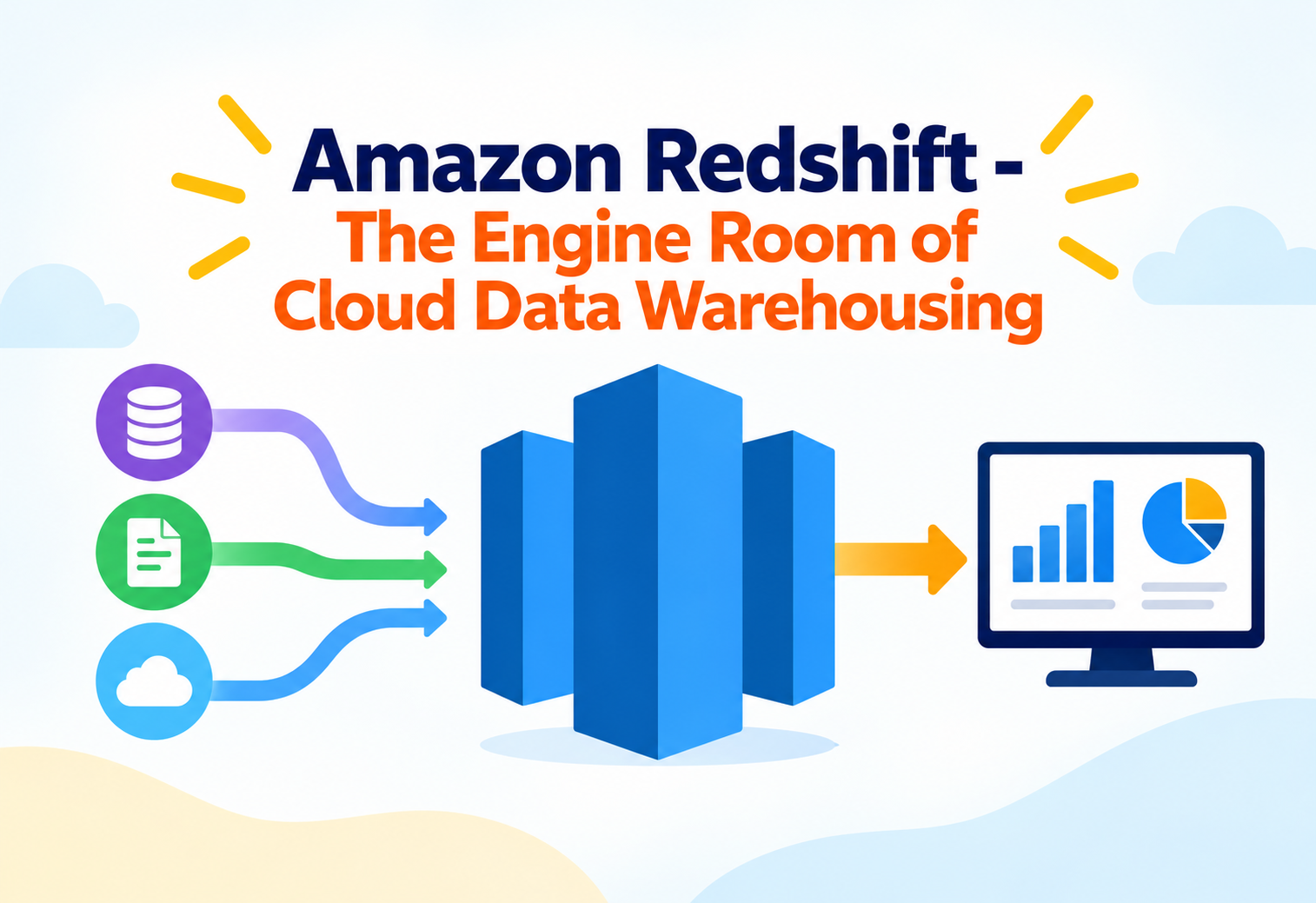
Amazon Redshift – The Engine Room of Cloud Data Warehousing
A deep, practical walkthrough of how Redshift stores, distributes, and queries petabytes of data — and how to reason about it like the engineers who run it in production.
Imagine a library so large that a single librarian could never answer every question fast enough — questions like “how many books were checked out on rainy Tuesdays in the last five years?” To answer that quickly, you don’t hire one very fast librarian. You hire a hundred librarians, split the shelves between them, and have each one search their own section at the same time. That, in a sentence, is the idea behind Amazon Redshift. It is a cloud data warehouse — a system built not to store a few records at a time, but to sift through billions of rows and hand back an answer in seconds. This guide assumes you already know the basics of what a data warehouse is; instead, it goes into the intermediate mechanics that separate someone who has “used Redshift” from someone who understands why it behaves the way it does.
1Introduction & History
Amazon Redshift launched in 2012, and it changed the economics of data warehousing almost overnight. Before Redshift, running a data warehouse meant buying specialized, expensive appliances from vendors like Teradata or Oracle Exadata — hardware that could cost hundreds of thousands of dollars before you had loaded a single row of data. AWS took a different bet: build a warehouse as a cloud service, priced by the hour, that could be provisioned in minutes instead of months.
Under the hood, Redshift is based on ParAccel, a columnar, massively parallel processing (MPP) database technology that AWS licensed and then rebuilt extensively. Think of ParAccel as the blueprint AWS started from, the way a car company might start from a chassis design before building its own engine, dashboard, and software around it. Over the years, Redshift has moved far beyond that starting point — introducing its own storage layer (RA3 with managed storage on Amazon S3), a serverless deployment option, and deep integration with the rest of the AWS data ecosystem.
Think of traditional on-premises data warehouses as owning a fleet of delivery trucks outright — you pay for them whether you use them or not, and scaling up means buying more trucks and waiting for delivery. Redshift is more like a truck rental service: you request capacity when you need it, pay for what you use, and can scale from one truck to a hundred in the time it takes to place an order.
A concrete example: Nasdaq migrated large portions of its market-surveillance analytics to Redshift specifically to avoid the capacity-planning headaches of fixed hardware — during periods of high trading volume, the workload could scale without a multi-month hardware procurement cycle. That single design choice — decoupling “I need a data warehouse” from “I need to buy a machine” — is the reason Redshift exists at all.
2Problem & Motivation
Relational databases like PostgreSQL or MySQL are built and optimized for transactional workloads: inserting a new order, updating a customer’s address, checking a single account balance. These are called OLTP (Online Transaction Processing) systems, and they are extremely good at touching a small number of rows very quickly, many times per second.
Analytics is the opposite kind of problem. A question like “what was our average order value by region, by month, for the last three years?” doesn’t touch one row — it has to scan millions or billions of rows, and it does this occasionally rather than constantly. This is called OLAP (Online Analytical Processing). If you tried to run OLAP-style queries against a normal OLTP database at scale, two things go wrong: the query is slow because the database has to read entire rows off disk even though it only needs two or three columns out of dozens, and the query competes for the same resources that customer-facing transactions need, potentially slowing down your live application.
This OLTP-versus-OLAP split is one of the most common interview and design-review topics in data engineering. If someone proposes running heavy analytics directly against a production transactional database, the correct instinct is to separate the workloads — which is exactly the gap Redshift is built to fill.
Redshift’s answer to this problem has two parts. First, it stores data by column rather than by row (explained in detail in the next chapter), so a query that only needs three columns out of fifty never has to touch the other forty-seven. Second, it spreads the data and the work across many machines at once, so instead of one processor reading a billion rows sequentially, a hundred processors each read ten million rows in parallel.
3Core Concepts (Intermediate Level)
Columnar Storage in Practice
In a row-oriented database, all the values for one record are stored together on disk — first name, last name, order date, amount, all packed side by side. In Redshift, data is stored by column instead: every value for “order date” across every row sits together, separately from every value for “amount.” The practical effect is that a query scanning only two columns out of forty physically reads a fraction of the data from disk, and because values in a single column tend to be similar to each other, they compress far better than mixed row data — often five to ten times smaller.
Distribution Styles
Because Redshift spreads a table’s rows across multiple compute nodes, you have to decide how those rows get divided up. This is the distribution style, and it is one of the most consequential design decisions in a Redshift schema.
Distribution by Column
Rows with the same value in a chosen column (e.g., customer_id) always land on the same node slice. This makes joins on that column fast because matching rows are already co-located.
Round-Robin Distribution
Rows are spread evenly across nodes regardless of content. Good for tables that aren’t frequently joined, since it guarantees balanced load but no co-location benefit.
Full Copy Everywhere
A full copy of the table is stored on every node. Ideal for small, frequently joined lookup or dimension tables — no data movement is needed at join time.
Redshift Decides
Redshift automatically chooses and can even change the distribution style as a table grows, starting small tables as ALL and switching larger ones to EVEN or KEY.
Picture four moving crews packing boxes for a house move. If you distribute by KEY on “room,” every crew member packing “kitchen” boxes works together at the kitchen — nothing needs to be handed across the house later. Distribute EVEN and boxes go to whichever crew member is free, which is fair on effort but means kitchen items end up scattered across every truck, so you’ll need to re-sort them at the new house. That re-sorting is exactly what Redshift has to do at query time when a join requires data that isn’t co-located — it’s called data redistribution, and it is one of the most common causes of slow queries.
Sort Keys
A sort key determines the physical order rows are stored in on disk within each node slice. Redshift supports compound sort keys, where columns are prioritized in order (useful when queries consistently filter on the first column, then narrow further with the second), and interleaved sort keys, which give equal weight to multiple columns so queries filtering on any one of them still benefit — at the cost of slower load and maintenance operations. A well-chosen sort key lets Redshift skip huge blocks of data entirely using zone maps: lightweight metadata that records the minimum and maximum value stored in each 1MB block, so if you filter for dates in March, Redshift can skip every block whose min/max range doesn’t include March without reading a single row.
Node Slices and Massively Parallel Processing (MPP)
Every compute node in a Redshift cluster is internally divided into slices — a slice is a portion of the node’s memory and disk allocated to process a subset of the workload. A table’s rows are distributed across all slices in the cluster, and when a query runs, each slice processes only its own portion of data simultaneously with every other slice, then the leader node combines the partial results. This is the core of MPP: instead of one big processor doing everything sequentially, many smaller processors do a fraction of the work at the same time.
4Architecture & Components
Every Redshift cluster has exactly one leader node and one or more compute nodes. The leader node is the receptionist and project manager combined: it accepts client connections, parses and optimizes incoming SQL, builds an execution plan, hands out pieces of that plan to the compute nodes, and finally assembles the partial results each compute node returns into a single answer for the client. The leader node does not store table data.
Compute nodes do the heavy lifting: each one holds a portion of every distributed table, executes the piece of the query plan the leader assigned to it, and has its own CPU, memory, and (for the older DC2 node family) local SSD storage. On the newer RA3 node family, which is the current recommended choice, compute and storage are decoupled — table data lives in a managed storage layer built on Amazon S3, and compute nodes cache the hot data they need locally while relying on high-speed networking to fetch anything not already cached. This decoupling is what allows RA3 clusters to scale compute and storage independently, rather than being forced to add expensive compute nodes just to get more disk space.
Redshift Spectrum extends this architecture further by allowing compute nodes to query data sitting directly in Amazon S3 — in open formats like Parquet, ORC, or CSV — without first loading it into the cluster, using a separate fleet of Spectrum compute resources that scale independently from your cluster’s own nodes.
A common question is “why does Redshift separate a leader node from compute nodes instead of having every node do everything?” The expected answer: centralizing query planning avoids the coordination overhead of every node negotiating a plan independently, and it lets AWS charge for compute capacity (nodes) separately from the always-on coordination role.
5Internal Working
When you submit a query, the leader node’s query optimizer first rewrites and simplifies the SQL, then generates several candidate execution plans and picks the one it estimates will be cheapest, using statistics about table size and data distribution gathered by the ANALYZE command. The chosen plan is compiled into C++ code and then into machine code — a step called code generation — rather than being interpreted step by step. This compilation step is why the very first time a particular query “shape” runs on a cluster it can feel slower: Redshift caches compiled code so subsequent similar queries skip recompilation.
The compiled plan is segmented into steps that get pushed down to every compute node slice, each of which executes against its own local (or cached, for RA3) columnar data. If a join or aggregation requires rows that live on a different slice than expected — because the distribution style doesn’t align with the join key — Redshift performs a data redistribution step, physically moving rows between slices over the cluster’s internal network before the join can complete. This redistribution is invisible in the SQL you write but very visible in query latency, which is why distribution-style design matters so much.
Compiling a query plan is like a chef prepping a recipe once at the start of a busy night: chopping vegetables and organizing stations up front is slower for the very first order, but every order after that flows through the same prepped stations quickly. Redshift is willing to pay that first-order cost once and amortize it across every similar order that follows.
Workload Management (WLM) governs how many queries can run concurrently and how memory is divided among them. In Auto WLM mode — the default and recommended setting — Redshift dynamically allocates memory and concurrency per query queue based on the nature of the workload, rather than requiring an administrator to hand-tune fixed queue slots. Short Query Acceleration (SQA) detects short-running queries and routes them to a dedicated queue so a handful of small dashboard queries never get stuck waiting behind one enormous batch job.
6Data Flow & Lifecycle
Data almost never trickles into Redshift row by row. The recommended pattern is bulk loading using the COPY command, which reads files in parallel directly from Amazon S3 (or streams from Kinesis Data Firehose, or is migrated via AWS Database Migration Service) and distributes the load work across all compute node slices simultaneously. Loading data with individual INSERT statements is dramatically slower because each one is a separate transaction with its own overhead — the difference in throughput between COPY and row-by-row INSERT can be well over a hundredfold at scale.
After loading, two maintenance operations keep a table healthy. VACUUM reclaims space from deleted or updated rows (Redshift’s storage engine marks old versions of rows rather than overwriting them in place, similar in spirit to MVCC in PostgreSQL) and re-sorts data according to the sort key. ANALYZE refreshes the statistics the query optimizer relies on to estimate row counts and choose good execution plans; skipping ANALYZE after a large load is one of the most common causes of a query optimizer picking a bad plan. Since Redshift’s Auto Vacuum and Auto Analyze features run these automatically in the background for most workloads today, manual invocation is now mostly reserved for large one-off loads where you want control over timing.
7Advantages, Disadvantages & Trade-offs
Advantages
- Massively parallel, columnar engine handles billions of rows with sub-minute (often sub-second) response for well-designed queries
- RA3 decouples storage from compute, so storage grows without forcing you to buy more compute
- Deep native integration with S3, Glue, Kinesis, SageMaker, and QuickSight reduces data-movement plumbing
- Serverless option removes cluster sizing decisions entirely for variable or spiky workloads
- Redshift Spectrum lets you query S3 data lakes without a separate load step
Disadvantages / Trade-offs
- Not designed for OLTP — single-row lookups and frequent small updates are inefficient compared to a transactional database
- Poor distribution-key or sort-key choices can silently degrade performance without any error being raised
- Provisioned clusters require capacity planning; under-provisioning causes queueing, over-provisioning wastes spend
- Concurrency at extreme scale still requires careful WLM/Concurrency Scaling configuration
- Vendor lock-in: while it speaks a PostgreSQL-derived SQL dialect, it is not a drop-in PostgreSQL replacement
The trade-off underneath almost every Redshift design decision is between flexibility for varied query patterns and optimization for a specific, known pattern. A perfectly chosen distribution and sort key can make one dominant query blazingly fast while making an unanticipated ad-hoc query on a different column noticeably slower — there is no single configuration that is optimal for every possible query.
8Performance & Scalability
Redshift offers three distinct ways to scale, and understanding when to use each is an intermediate-level skill in itself. Elastic resize changes the number or type of nodes in a cluster in minutes by redistributing data across the new node count, with a brief period of read-only or unavailable access; it is meant for planned, relatively infrequent capacity changes. Classic resize is the older, slower method that creates a new cluster and copies data over, used for changes elastic resize can’t handle, such as certain node-type migrations. Concurrency Scaling automatically spins up additional, transient clusters within seconds to absorb bursts of concurrent read queries, then shuts them back down when the burst passes, billing only for the burst usage.
Materialized views pre-compute and store the result of a query, refreshing incrementally when possible, which is especially effective for dashboards that repeatedly run the same aggregation over data that changes slowly. Result caching goes a step further for identical repeated queries by returning a cached answer from the leader node instantly, bypassing compute nodes entirely, as long as the underlying data hasn’t changed.
Amazon Redshift Serverless removes the node-count decision altogether: you set a base and maximum Redshift Processing Unit (RPU) range, and the service scales compute up and down automatically based on workload, billing per RPU-second of usage. This is a strong fit for workloads with unpredictable or intermittent query patterns, such as a startup whose analytics traffic is heavy during business hours and near zero overnight, since a provisioned cluster sized for the daytime peak would sit mostly idle — and therefore mostly wasted — every night.
9High Availability & Reliability
A Redshift cluster is deployed within a single Availability Zone by default, but the service continuously monitors node health and automatically replaces a failed compute node, restoring its data from the RA3 managed storage layer or from replicated data on other nodes, without requiring manual intervention. For higher resilience, Multi-AZ deployments (available for RA3 clusters) run compute across two Availability Zones, so an entire AZ outage doesn’t take the cluster fully offline.
Automated snapshots are taken periodically and incrementally, capturing only changed data blocks since the last snapshot to minimize storage cost and time, and can be configured to copy cross-region for disaster recovery. Because RA3’s actual data lives in the managed storage layer on S3 — itself designed for eleven nines of durability — the durability story for Redshift is inherited in large part from S3’s own guarantees, with compute nodes treated as replaceable, stateless-ish workers relative to that durable base layer.
“If a compute node fails mid-query, what happens to that query?” The expected answer: the query typically fails and must be retried by the client or the application layer, since Redshift does not transparently resume a query on a replacement node mid-execution — reliability here is about the cluster recovering quickly, not about individual in-flight queries surviving a node failure.
10Security
Redshift clusters are typically launched inside an Amazon VPC, isolated from the public internet by default, with security groups controlling exactly which network sources can reach the cluster’s port. Enhanced VPC Routing forces all data-loading and unloading traffic (COPY/UNLOAD to and from S3) through the VPC rather than over the public AWS network path, which matters for organizations with strict network-egress compliance requirements.
Encryption is available at two layers: in transit, connections can be forced to use SSL/TLS; at rest, cluster data can be encrypted using AWS Key Management Service (KMS) keys, either AWS-managed or customer-managed, and RA3’s managed storage layer inherits S3’s own server-side encryption capabilities. Authentication and access control layer on top of this: IAM roles attached to the cluster grant it permission to read from S3 or write logs, database-level users and groups control who can query which schemas and tables, and column-level and row-level security let administrators restrict access to sensitive columns (like a salary field) or specific rows (like restricting a regional manager to only their region’s data) without maintaining separate copies of the table for each audience.
Row-level and column-level security work like giving every employee the same building keycard but programming different doors to open for different badges — everyone walks through the same front entrance (the same table), but what they can actually see or unlock once inside varies by their role.
Every user action and system event can be captured through database audit logging and AWS CloudTrail, which records API-level actions against the cluster (like resizing or snapshotting) for compliance and forensic review.
11Monitoring, Logging & Metrics
Amazon CloudWatch collects cluster-level metrics — CPU utilization, disk space used, database connections, query throughput, and Concurrency Scaling usage — and can trigger alarms when thresholds are crossed, such as notifying an on-call engineer when disk usage crosses eighty percent. Inside the database itself, system views and system tables (prefixed STL, STV, SVL, and SVV) expose detailed query history, including which queries ran, how long each execution step took, and whether any step spilled to disk because it ran out of allocated memory.
Amazon Redshift Advisor analyzes a cluster’s usage patterns automatically and surfaces specific, actionable recommendations — for example, flagging a table whose actual distribution style doesn’t match its query patterns, or identifying tables that would benefit from compression encoding changes. Query Monitoring Rules (QMR), configured as part of WLM, can automatically log, hop to another queue, or abort a query that violates a defined rule, such as one that has been running longer than a defined threshold or is consuming an excessive share of memory — a useful safety net against a single runaway analyst query starving the rest of the cluster.
12Deployment & Cloud Integration
Provisioning happens through the console, the AWS CLI, CloudFormation, or Terraform, letting a data platform team define cluster configuration as version-controlled infrastructure rather than manual clicks. Redshift Serverless simplifies this further by removing node-count and node-type decisions from the provisioning step entirely.
Redshift’s integrations form much of its practical value: the Redshift Data API allows applications to run SQL against a cluster over HTTPS without managing persistent database connections, which fits well with serverless application architectures like AWS Lambda. AWS Glue and Amazon EMR commonly write transformed data into S3 for Redshift to load or query via Spectrum. Federated Query lets Redshift reach directly into operational databases like Amazon Aurora or RDS PostgreSQL to join live transactional data with warehoused analytical data in a single query, without a separate ETL step to copy that data first. Data Sharing allows one Redshift cluster to securely share live access to specific databases with another Redshift cluster or account — including across AWS accounts — without physically copying or moving the underlying data, which is particularly useful for a data-producing team sharing curated datasets with multiple consuming teams.
13Design Patterns & Anti-Patterns
Context
A large fact table (e.g., order line items) needs to join frequently against several smaller dimension tables (e.g., customers, products, dates).
Pattern
Distribute the fact table by KEY on the most frequently joined column, and set small dimension tables to ALL distribution so a full copy exists on every node — eliminating redistribution during the join entirely.
Symptom
Queries joining a large fact table to a dimension table are slow, and the query plan shows a significant redistribution step consuming most of the execution time.
Root Cause
EVEN distribution scatters rows without regard to join keys, so almost every join has to shuffle data across the network before it can proceed — the opposite of what KEY distribution achieves for the same join.
Symptom
Loads and VACUUM operations become dramatically slower over time as a table grows.
Root Cause
Interleaved sort keys maintain a balanced ordering across multiple columns simultaneously, which is more expensive to update on every load; using more than three or four interleaved columns, or applying interleaving where a simple compound key would do, is a frequent, avoidable source of maintenance overhead.
14Best Practices & Common Mistakes
- Load in bulk, not row by row. Always prefer COPY from S3 over individual INSERT statements for anything beyond trivial data volumes.
- Right-size distribution keys deliberately. Choose the column used in the largest, most frequent joins — not simply the primary key out of habit.
- Don’t skip ANALYZE after large loads if Auto Analyze is disabled or delayed; stale statistics are a leading cause of unexpectedly slow queries.
- Use compression encodings deliberately. Letting Redshift’s COPY command auto-select encodings on initial load is usually a safe default; revisit only when profiling shows a specific column is a storage or scan bottleneck.
- Separate workload queues for ETL/batch jobs versus interactive BI queries so a long-running transformation job doesn’t starve a dashboard refresh.
- Common mistake: treating Redshift like an OLTP database by issuing frequent single-row UPDATE or DELETE statements, which fight against the columnar, append-oriented storage model.
- Common mistake: over-provisioning “just in case.” Concurrency Scaling and elastic resize exist precisely so teams don’t need to permanently size a cluster for rare peak moments.
15Real-World & Industry Examples
Nasdaq — Market Surveillance at Scale
Nasdaq uses Redshift to analyze massive volumes of trading data for market-surveillance purposes, relying on the ability to scale compute during periods of unusually high trading activity without pre-provisioning permanent hardware sized for worst-case volume.
McDonald’s — Global Operational Analytics
McDonald’s has used Redshift as part of its cloud data platform to consolidate operational and sales data across thousands of locations globally, enabling faster, more consistent reporting than region-by-region, siloed reporting systems allowed previously.
Yelp — Ad Analytics and Business Insights
Yelp has publicly discussed using Redshift as a core piece of its data warehousing stack for advertising analytics, feeding business-facing dashboards used by both internal teams and business owners reviewing their own performance metrics.
16Frequently Asked Questions
17Summary & Key Takeaways
Key Takeaways
- Redshift is a columnar, massively parallel processing (MPP) cloud data warehouse purpose-built for analytical (OLAP) queries over huge datasets, not transactional (OLTP) workloads.
- A leader node plans and coordinates queries; compute nodes, divided into slices, do the actual parallel work against locally cached or stored columnar data.
- Distribution style (KEY, EVEN, ALL, AUTO) and sort keys are the two most consequential schema decisions, directly determining whether joins require expensive data redistribution.
- RA3 node types decouple compute from storage via a managed layer on Amazon S3, allowing independent scaling of each.
- Elastic resize, classic resize, Concurrency Scaling, and Redshift Serverless each solve a different scaling problem — planned capacity change, structural node-type change, sudden concurrent-query bursts, and fully automatic sizing, respectively.
- Security is layered: VPC network isolation, encryption in transit and at rest via KMS, IAM-based access, and fine-grained column- and row-level controls.
- Common failure modes are almost always design mistakes, not the engine itself — poor distribution keys, skipped statistics refreshes, or treating Redshift like a transactional database.