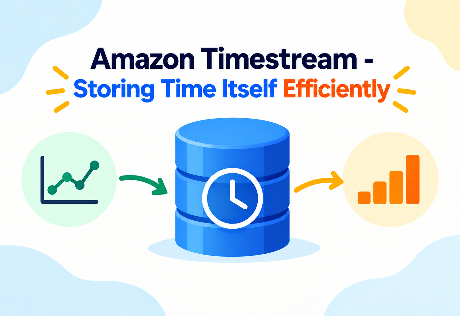
Amazon Timestream became generally available in 2020, arriving several years after open-source time series databases like InfluxDB and Prometheus had already proven there was strong demand for storage engines specialized around timestamped data. AWS’s pitch was distinct from those tools in one specific way: full serverless operation. Where InfluxDB or Prometheus typically require you to size, patch, and scale servers yourself, Timestream was designed from day one to automatically scale storage and compute independently, with no clusters, nodes, or shards to manage.

More recently, AWS expanded the Timestream family by launching Timestream for InfluxDB, a fully managed service running the actual open-source InfluxDB engine for teams that want InfluxQL/Flux compatibility, alongside the original service — now referred to as Timestream for LiveAnalytics — which uses its own SQL-based query engine. This guide focuses on Timestream for LiveAnalytics, the original and most widely deployed variant.

A concrete example: Samsung SmartThings uses Timestream to store and analyze telemetry data from millions of connected smart-home devices, a workload defined almost entirely by high-volume, continuous writes and time-windowed reads — precisely the pattern Timestream was purpose-built to absorb.

Time series workloads have a distinctive shape that breaks the assumptions most databases are optimized around. Writes are almost always new inserts — you rarely go back and update a temperature reading from three days ago — and they arrive at extremely high volume and frequency, sometimes millions of data points per second across many devices. Reads, meanwhile, are almost always scoped to a time window: “show me the last 24 hours,” “compare this week to last week,” “give me the average per minute for the last hour.”

A general-purpose relational database struggles with this pattern for a structural reason: it typically has no built-in concept that recent data is accessed constantly while old data is accessed rarely, so it stores and indexes everything the same way regardless of age. That means you either pay premium storage and compute costs to keep years of rarely touched historical data on the same expensive infrastructure as this morning’s hot data, or you build your own manual archiving pipeline to move old data elsewhere — extra engineering effort that has nothing to do with your actual application.

Timestream’s answer is to build that tiering directly into the database itself, rather than leaving it as an application-level concern, and to price storage and compute for each tier differently, so the cost model naturally rewards the “recent data is hot, old data is cold” access pattern instead of fighting against it.

The Data Model: Dimensions, Measures, and Records

A record in Timestream is a single data point, and it has three kinds of fields. Dimensions are attributes that describe the source of the data and rarely change for a given entity — for example, device_id, region, or sensor_type. Measures are the actual values being recorded — temperature, cpu_utilization, heart_rate — along with a measure name and a data type (BIGINT, DOUBLE, VARCHAR, BOOLEAN, or TIMESTAMP). Every record also has a timestamp indicating when the measurement occurred, plus a time unit of precision (from nanoseconds to seconds).

Single-Measure vs. Multi-Measure Records

Early Timestream tables stored one measure per record, meaning a device reporting both temperature and humidity at the same instant produced two separate records sharing the same dimensions and timestamp. Multi-measure records, introduced later, allow multiple related measures to be packed into a single record instead — so one row can hold temperature, humidity, and pressure together under one timestamp. This matters for two reasons: it reduces the number of records (and therefore ingestion and storage cost) for sources reporting several correlated values at once, and it makes queries that need several measures at the same point in time simpler to write, since they no longer require joining separate rows back together.

Memory Store and Magnetic Store

Every Timestream table is really backed by two storage tiers working together. The memory store holds the most recent data — the window is configurable, commonly ranging from minutes to a couple of weeks — in a layout optimized for very fast writes and very fast recent-data queries. Data automatically migrates out of the memory store into the magnetic store once it ages past the configured retention window, where it is compressed and stored far more cost-effectively for long-term retention, often for months or years, while remaining fully queryable through the exact same SQL interface.

Adaptive Query Processing

Because a single query can span data living in both the memory store and the magnetic store, Timestream’s query engine performs adaptive query processing — it determines which store(s) a query actually needs to touch based on the time range in the query’s WHERE clause, and it can push filtering and even partial aggregation down closer to the storage layer rather than pulling all matching raw rows up to a central node first. A query scoped only to “the last hour” never touches the magnetic store at all, which keeps common recent-data queries fast regardless of how much historical data the table has accumulated overall.

Timestream has no user-visible servers, clusters, or nodes to configure. The ingestion and routing layer accepts writes through the WriteRecords API, validates and batches incoming records, and lands them in the memory store for the table they belong to. As data ages past the memory store’s configured retention window, a background process automatically migrates it to the magnetic store, compressing it in the process.

The query layer sits logically above both stores and exposes a single SQL interface, so an application or BI tool never needs to know or care whether the rows it’s asking for live in the memory store, the magnetic store, or span both — that decision is made internally, transparently, by the query engine’s adaptive processing.

When a write arrives via the WriteRecords API, Timestream validates the record against the table’s schema expectations, checks the timestamp against the memory store retention window (records too far outside the allowed window are rejected, since they don’t logically belong in either tier’s current configuration), and appends the record. Because writes are almost always new inserts along an increasing timestamp, Timestream’s internal storage layout for the memory store is optimized around this append-heavy, time-ordered access pattern rather than the general-purpose update-in-place patterns a transactional database has to support.

On the query side, the SQL parser translates a query into an execution plan, and the adaptive query processing layer inspects the time predicates in that plan to determine which store(s) actually hold data satisfying the time range. If a query only asks for “the last 10 minutes,” the engine can skip the magnetic store’s compressed data files entirely; if a query spans “the last 6 months,” the engine must combine data from both stores and merge the results. Time series-specific SQL functions — including interpolation (filling in gaps between irregular readings), smoothing, and approximate aggregation functions for high-cardinality data — are executed as part of this same query engine, so common time series analysis operations don’t require pulling raw data out into a separate application for post-processing.

A typical record’s life begins at the source — an IoT sensor, an application emitting metrics, or a Kinesis stream aggregating events from many producers — and is written via the WriteRecords API, often in batches to improve throughput efficiency, since batching amortizes the per-call overhead across many records at once. From there, the record lives in the memory store for as long as its table’s memory store retention period allows, fully queryable at low latency the entire time.

Once a record ages past that retention window, Timestream automatically migrates it to the magnetic store, applying compression that meaningfully reduces its storage footprint. The record remains queryable via the same SQL surface indefinitely, governed now by the table’s magnetic store retention period, until it finally ages past that longer window and is deleted automatically. This entire lifecycle — hot storage, automatic aging, compressed cold storage, eventual expiry — happens without any scheduled jobs, Lambda functions, or manual scripts required from the application team; it is configured once, per table, as retention settings.

You may likeAmazon ECR→

The core trade-off is specialization itself: Timestream is excellent precisely because it refuses to be a general-purpose database, but that same specialization means forcing a non-time-series workload into it fights the engine rather than working with it.

Because Timestream is serverless, scaling is largely automatic rather than something engineers configure directly: write throughput and query concurrency scale up transparently to absorb increased load, and storage capacity grows without any provisioning step at all. This is a meaningful shift from provisioned time series databases, where a sudden spike in device count or reporting frequency would otherwise require manually resizing infrastructure ahead of time.

Practical performance still depends on schema design choices: choosing sensible dimensions (attributes you’ll filter or group by) versus measures (values you’re recording) affects both storage efficiency and query plan quality, and using multi-measure records where multiple values genuinely share a timestamp and source reduces both ingestion volume and the number of joins a query needs to perform. Scheduled queries — a feature that runs a saved query on a defined interval and writes the result back into another table — are a common pattern for pre-aggregating expensive, wide-time-range queries (like daily rollups) so that dashboards querying the rollup table stay fast even as the underlying raw data volume grows.

As a fully managed AWS service, Timestream replicates data across multiple Availability Zones within a region automatically, without requiring the customer to configure replication settings, failover logic, or standby infrastructure. This differs meaningfully from a self-managed time series database, where achieving multi-AZ durability would require deliberately architecting and testing a replication topology.

Because there are no individual nodes for a customer to monitor or fail over manually, reliability from the customer’s perspective is largely expressed through service availability guarantees and automatic recovery behavior rather than through visible infrastructure health metrics — the operational burden of “what happens if a node dies” is absorbed by AWS rather than surfaced to the application team.

Access to Timestream databases and tables is controlled through AWS IAM policies, which can be scoped down to specific actions (like WriteRecords or Select) and even specific databases or tables, so a device-ingestion role can be granted write-only access while a dashboard’s read role has no write permissions at all. Data at rest is encrypted using AWS Key Management Service (KMS), and connections to the service are encrypted in transit using TLS.

For workloads that must avoid traversing the public internet, VPC endpoints allow applications running inside a VPC to reach Timestream privately, keeping traffic on the AWS network backbone rather than exposed to the public internet path. Because Timestream is often fed by IoT devices at the network edge, security design frequently focuses as much on securing the ingestion path — device certificates, IoT Core policies, and constrained IAM roles for the services relaying data — as on the database itself.

Amazon CloudWatch collects Timestream-specific metrics, including successful and failed write record counts, query latency, and data ingestion volume, letting teams alarm on issues like a sudden spike in rejected writes — often the first visible sign that devices are sending timestamps outside the configured memory store retention window. AWS CloudTrail logs management-level API calls against Timestream, such as table creation or retention policy changes, supporting audit and compliance needs.

Because Timestream integrates natively with Amazon Managed Grafana and Amazon QuickSight, many teams build their primary operational dashboards directly against these tools rather than a custom monitoring layer, querying Timestream tables with the same SQL interface used for application queries.

Databases and tables can be created through the console, AWS CLI, CloudFormation, or Terraform, with retention periods for both the memory store and magnetic store defined as table-level configuration rather than infrastructure to provision. Because there’s no cluster to size, “deployment” in the traditional infrastructure sense is largely reduced to schema and retention-policy design.

Timestream integrates closely with the rest of AWS’s IoT and streaming ecosystem: AWS IoT Core can route device telemetry directly into Timestream through an IoT rule, Amazon Kinesis Data Streams and Kinesis Data Firehose can buffer and batch high-volume event streams before writing them in, and AWS Lambda functions commonly sit in the ingestion path to transform or enrich incoming data before it’s written. On the consumption side, Grafana and QuickSight connect natively for visualization, and general SQL clients can connect via JDBC/ODBC drivers for ad-hoc analysis.

You may likeAmazon ECS→

• Plan memory store retention around your worst realistic data-arrival delay, not the typical case, to avoid unexpected write rejections from late-arriving records.
• Use multi-measure records whenever multiple values genuinely share a timestamp and source, rather than defaulting to single-measure records out of habit.
• Batch writes through the WriteRecords API rather than issuing one API call per individual data point, to reduce per-call overhead at high volume.
• Pre-aggregate expensive, wide-range queries with scheduled queries instead of recomputing them from raw data on every dashboard refresh.
• Common mistake: treating dimensions and measures interchangeably, which leads to awkward schemas — dimensions should be the relatively stable attributes you filter or group by, measures should be the values actually being recorded.
• Common mistake: forcing frequently updated or heavily relational data into Timestream, when a transactional or general-purpose database would fit that access pattern far better.