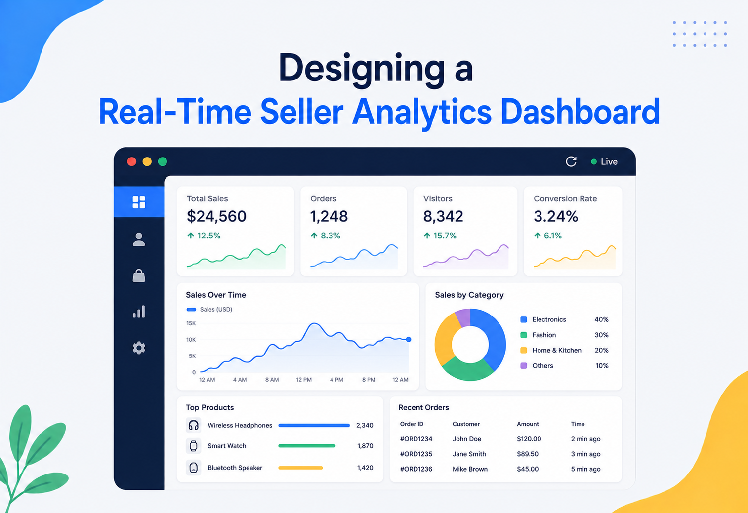
Designing a Real-Time Seller Analytics Dashboard
A complete, from-first-principles walkthrough of how large marketplaces build systems that give millions of independent sellers a live view of their own sales, traffic, and conversion metrics — updated in near real time, accurate down to the last order, and fast enough to feel instantaneous even under enormous concurrent load.
Introduction & History
Log into a large marketplace as a seller today, and you are met with a dashboard: sales climbing through the day, a conversion rate updating as shoppers browse and buy, traffic numbers ticking upward during a promotion. For the seller, this feels almost like watching a live scoreboard. Underneath that scoreboard sits one of the more demanding categories of system to build well — a real-time analytics platform that has to ingest an enormous, continuous stream of clickstream and order events across millions of sellers and products, and turn it into fast, accurate, per-seller metrics that update within seconds, not hours.
1.1 From nightly batch to live scoreboard
Business analytics itself is an old discipline. Traditional business intelligence systems, built through the 1990s and 2000s, ran nightly batch jobs that loaded the previous day’s transactions into a data warehouse, and analysts queried that warehouse the next morning. This was perfectly adequate for quarterly and monthly reporting, but it created a fundamental problem for anyone who needed to react quickly: a seller running a flash sale, or troubleshooting a sudden drop in conversion, could not afford to wait until tomorrow to find out what happened today.
The shift toward genuinely real-time analytics tracks closely with the rise of stream processing technology in the 2010s. Systems like Apache Kafka, and stream processing engines built to consume from it, made it practical to treat a continuous flow of events — page views, add-to-carts, completed orders — as a first-class data source that could be aggregated and queried within seconds of an event happening, rather than only after it had been batch-loaded overnight. Purpose-built real-time analytical databases, optimized specifically for fast aggregation queries over huge, constantly growing datasets, matured alongside this shift, and together these pieces are what made a live, per-seller dashboard at marketplace scale technically achievable.
Nightly Batch BI
Overnight ETL loaded yesterday’s transactions into a warehouse; analysts got answers the next morning. Fine for quarterly reviews, useless for anyone reacting to a live promotion.
Micro-Batches & Reporting Replicas
Scheduled jobs recomputed rollups every few minutes into a dedicated reporting store, and read replicas offloaded dashboard reads from the primary. Better freshness, but still not live and still not built for the aggregation shape.
Streaming + Real-Time OLAP
A durable event log (Kafka), a windowed stream processor, and a purpose-built OLAP store turn each event into an updated rollup within seconds — the design this guide is about.
Think of the difference between a store’s end-of-day cash register tape and a live scoreboard at a sports match. The cash register tape is accurate and complete, but you only get to read it after the store closes. A live scoreboard is being updated continuously as the game unfolds, giving the coach information they can actually act on while the game is still being played. A real-time analytics dashboard is the scoreboard; the nightly batch report it replaced was the cash register tape.
This guide focuses on that generation of systems: high-cardinality (millions of distinct sellers, each wanting their own slice of data), high-throughput (constant clickstream and order volume across the whole marketplace), and near-real-time, built on the same distributed systems building blocks used broadly across modern backend engineering — API gateways, load balancers, message queues, and purpose-built analytical stores — applied specifically to the problem of live, per-seller business metrics.
The Problem & Why a Naive Approach Fails
Before any architecture, it helps to be precise about why this is genuinely hard, because the naive approach — “just run a SQL query against the orders table whenever a seller opens their dashboard” — collapses almost immediately at real marketplace scale.
2.1 Aggregation over raw transactional data does not scale to this read pattern
A marketplace’s operational order database is optimized for writing and reading individual orders quickly and reliably, not for computing “total sales for seller X in the last hour” across potentially millions of rows, repeated continuously by millions of sellers checking their dashboards throughout the day. Running that kind of aggregation query live, against the same database handling live checkout traffic, would quickly degrade both the dashboard experience and, far more dangerously, the checkout experience itself.
2.2 Traffic and conversion data does not live in the order database at all
Sales figures come from completed orders, but traffic and conversion metrics need page views, product impressions, and add-to-cart events — a completely different, much higher-volume data source generated by the storefront itself, not the order system. A seller’s conversion rate is a ratio between two different event streams entirely, which already tells you this cannot be a single simple query against one table.
2.3 Millions of sellers means extreme cardinality
Unlike a single company’s internal analytics dashboard, a marketplace analytics system must serve a genuinely enormous number of distinct, independent “tenants” — every seller wants their own accurate, isolated view of their own data, and that data must never leak across sellers. Pre-computing and storing metrics broken down by seller, and often further broken down by product and time window, multiplies data volume dramatically compared to a single aggregate view of the whole marketplace.
2.4 “Real time” and “accurate” pull in different directions
A system that recomputes exact aggregates fast enough to feel live typically has to make some trade-off against perfect precision, especially at high event volume, while a system that guarantees perfectly exact results usually cannot do so within a few seconds at this scale. Handling this tension deliberately, rather than accidentally, is one of the defining design decisions covered throughout this guide.
Build a system that ingests continuous clickstream and order event volume across an entire marketplace, computes accurate, per-seller sales, traffic, and conversion metrics broken down by time window and product, and serves those metrics to millions of sellers through a dashboard that updates within seconds — without ever degrading the reliability or latency of the storefront and checkout systems that produce the underlying data.
“Why not just add a read replica to the orders database and query that for the dashboard?” A read replica helps isolate dashboard read load from the primary write path, which is a reasonable first step at small scale, but it does not solve the aggregation problem itself — a query computing rolling sums and conversion ratios across millions of rows, repeated by millions of concurrent sellers, will still be slow and expensive on a general-purpose relational replica, because that kind of database is not built for high-cardinality, high-concurrency aggregation queries the way a purpose-built analytical store is.
Core Concepts You Need First
Here is the shared vocabulary this guide relies on, each explained in plain language with a simple example.
3.1 Event
A single, timestamped fact — a page view, an add-to-cart, a completed order — that the system records as it happens. Every metric shown on the dashboard is ultimately derived from aggregating many of these raw events over some window of time.
3.2 Metric and dimension
A metric is a number you compute, such as total sales or session count. A dimension is a way of slicing that number, such as by seller, by product, or by hour. “Sales for seller X, by product, for today” is a metric sliced along two dimensions, and the combinatorial explosion of possible dimension combinations is a central design challenge for this kind of system.
Think of a metric as the number on a scoreboard, and dimensions as the different scoreboards you could build — one for the whole league, one per team, one per player. The underlying game events are the same; what changes is how you choose to slice and summarize them.
3.3 Time window / rollup
Rather than storing every raw event forever at full resolution, the system pre-aggregates events into fixed time buckets — per minute, per hour, per day — called rollups. A dashboard showing “sales this hour” reads a small number of pre-aggregated rollup rows instead of scanning potentially millions of raw events every single time someone looks.
3.4 Conversion rate
The ratio of a meaningful outcome, typically completed orders, to a preceding step, typically product views or sessions, over the same time window and dimension slice. Because it is a ratio between two independently arriving event streams, computing it correctly requires both streams to be aggregated consistently over matching time windows before the ratio is calculated.
3.5 Lambda and Kappa architecture
Two well-known architectural patterns for balancing real-time speed against long-term accuracy. A Lambda architecture runs two parallel pipelines: a fast “speed layer” that produces approximate, immediately available results, and a slower “batch layer” that recomputes exact results later and overwrites the approximate ones. A Kappa architecture simplifies this to a single stream-processing pipeline, treating reprocessing as just replaying the event log from an earlier point rather than maintaining two separate codebases. Both patterns show up directly in the architecture described later in this guide.
3.6 Tenant isolation
The guarantee that one seller’s dashboard queries, and one seller’s data, cannot be seen by or interfere with another seller’s, even though the underlying infrastructure is fully shared across all sellers for cost and operational efficiency.
3.7 Freshness SLA
An internal, measurable commitment for how quickly a raw event should be reflected in a seller’s dashboard — for example, “ninety-five percent of events visible within thirty seconds.” Defining this explicitly, rather than leaving “real time” as a vague aspiration, is what makes the speed layer’s performance measurable, testable, and something engineers can be alerted against when it slips.
3.8 Backfill
The process of recomputing rollups for a past time range, either because a bug in aggregation logic needs correcting retroactively, or because a new metric or dimension is being introduced that needs historical data populated before it can be shown on the dashboard. Because the raw event log is retained durably, a backfill is simply a matter of replaying historical events through the updated aggregation logic, which is one of the strongest practical arguments for always keeping the full raw event history rather than discarding it once rollups have been computed.

3.9 Vocabulary at a glance
| Term | What it answers | Typical data source |
|---|---|---|
| Raw event | What just happened? | Clickstream and order event streams |
| Rollup | What is the pre-aggregated summary for this time bucket? | Stream processor output |
| Conversion rate | What share of views turned into orders? | Ratio of two aggregated event streams |
| Speed layer result | What is the best available answer right now? | Real-time stream aggregation, approximate |
| Batch layer result | What is the exact, final answer? | Periodic recomputation over the full event log |
System Architecture & Components
With shared vocabulary in place, here is the full picture: the seller-facing read path that serves dashboard queries, and the ingestion and aggregation pipeline that continuously turns raw marketplace events into per-seller metrics.
4.1 Component-by-component breakdown
Below is what each labelled box in that diagram is actually responsible for, in plain terms.
CDN
Caches static dashboard assets close to the seller so only the dynamic metric queries themselves travel to the origin.
API Gateway
The single entry point for every dashboard request. Handles authentication, per-seller rate limiting, and routing to the correct backend service.
Load Balancer
Distributes dashboard query traffic across many identical Query Service instances using health checks, avoiding any single point of failure.
WebSocket Gateway
Maintains live, persistent connections to open dashboards so newly computed metrics can be pushed the moment they are ready, without the seller refreshing.
Query Service
The core read-path service; given a seller ID, time range, and requested metrics, returns pre-aggregated results, reading from cache first.
Aggregation Service
Consumes windowed output from the Stream Processor and writes finalized per-seller, per-dimension rollups into the OLAP store.
Alerting Service
Evaluates seller-configured thresholds, such as a conversion-rate drop, against fresh rollups and triggers live notifications.
Kafka Event Bus
Carries every clickstream and order event from the marketplace’s storefront and order systems into the analytics pipeline asynchronously.
Stream Processor
Continuously aggregates raw events into windowed metrics per seller and dimension, the computational heart of the speed layer.
Real-Time OLAP Store
A purpose-built analytical database storing pre-aggregated rollups, optimized for fast, high-concurrency aggregation queries.
Redis Cache
Stores the most frequently requested dashboard queries so repeated identical requests almost never have to hit the OLAP store directly.
Data Warehouse
The batch layer; periodically recomputes exact metrics over the full event history and reconciles them against the speed layer’s approximate results.
“Why do we need both an API Gateway and a Load Balancer here?” The API Gateway operates at the application layer, handling authentication, request validation, and routing across many different backend services beyond just analytics — order management, seller onboarding, and so on. The Load Balancer sits specifically in front of the Query Service fleet, distributing load across many stateless instances of that one service for scalability and fault tolerance. The two are complementary layers serving different purposes, not substitutes for one another.
4.2 Networking considerations
Services within the Analytics Core and Event Backbone layers communicate over a private virtual network, isolated from the public internet, with only the API Gateway and WebSocket Gateway exposed publicly. Connection pooling matters heavily between the Query Service and the OLAP store, since establishing a fresh connection on every dashboard request would add meaningful overhead at the concurrency this system operates under; persistent, pooled connections avoid that cost entirely. Service discovery lets the Query Service, Aggregation Service, and Alerting Service locate healthy instances of their dependencies dynamically as each fleet scales up and down independently, rather than relying on static, manually maintained address lists that would quickly go stale in an autoscaling environment.
4.3 Why the WebSocket Gateway is a separate component
It might seem simpler to have the Query Service itself hold WebSocket connections directly, but separating this concern is deliberate. Long-lived WebSocket connections have a fundamentally different resource profile than short, stateless request-response calls — many open, mostly idle connections held in memory over long periods, rather than many brief, independent requests. Isolating this into its own fleet means the Query Service can scale purely based on query throughput, while the WebSocket Gateway scales based on concurrent connection count, and a spike in one dimension never forces unnecessary scaling of the other.
Internal Working: From Raw Event to Live Metric
It helps to separate this system into two paths that run at very different speeds: the ingestion and aggregation path, which continuously turns a firehose of raw events into pre-computed metrics, and the read path, which serves an already-computed metric to a seller’s dashboard in milliseconds.
5.1 The ingestion and aggregation path
Every relevant marketplace event — a product page view, an add-to-cart, a completed order — is published to Kafka the moment it happens, tagged with the seller ID and product ID it belongs to. The Stream Processor consumes these events continuously, grouping them into small time windows, typically a minute or less, and computing partial aggregates within each window: event counts, sum of order values, and so on, broken down by seller and product. The Aggregation Service takes these partial window results and merges them into the OLAP store’s rollup tables, at multiple granularities simultaneously — per minute for the live dashboard’s most recent view, and per hour and per day for longer historical ranges.
5.2 The read path
When a seller opens their dashboard, the request never triggers a live scan over raw events. The Query Service translates the requested time range and metrics into a small number of rollup lookups against the OLAP store, which was purpose-built to answer exactly this kind of query — “sum of sales for seller X, per hour, for the last 24 hours” — extremely fast, since it is reading pre-aggregated rows rather than computing the aggregation on demand. A Redis cache sits in front of the most commonly repeated queries, such as “today so far,” to avoid even the OLAP store’s very fast query cost for the highest-traffic dashboard views.
5.3 Reconciling speed and accuracy
The rollups produced by the Stream Processor in real time are necessarily based on events seen so far, and a small number of events can arrive late due to network delays or upstream retries. Rather than blocking the live dashboard on perfect completeness, the system shows the best available real-time numbers immediately, and a periodic batch job recomputes exact totals from the complete, ordered event log in the Data Warehouse, correcting any small discrepancies after the fact. This is the Lambda architecture pattern introduced earlier, applied concretely.
Here is a simplified Java implementation of the core windowed aggregation logic, written the way it might appear inside the Stream Processor.
public class SalesAggregator {

    public void process(OrderEvent event, TimeWindow window) {
        AggregationKey key = new AggregationKey(
                event.getSellerId(), event.getProductId(), window.getBucketStart());

        MetricAccumulator acc = accumulatorStore.getOrCreate(key);
        acc.addSalesAmount(event.getOrderTotal());
        acc.incrementOrderCount();

        if (window.isReadyToFlush()) {
            RollupRow row = acc.toRollupRow(key, window);
            rollupWriter.upsert(row); // merges into existing rollup if one exists
        }
    }
}
The speed layer and batch layer work like a weather forecaster giving you today’s forecast now, based on the best current data, while a full climate scientist later reviews complete satellite records to publish the exact, corrected record for that day. Both are useful; you just need to know which one you are looking at.
“A seller says their dashboard shows fewer sales than what actually happened this hour. Is this a bug?” Not necessarily — this is expected, bounded behavior in a Lambda-style architecture if only a small number of late-arriving events have not yet been incorporated into the live rollup. The correct response is explaining the reconciliation window: the batch layer will correct any such small discrepancy within its next run, and the real concern is only if the gap is large or persists well past that reconciliation window, which would indicate an actual pipeline problem rather than expected eventual consistency.
5.4 A complete worked example
It helps to trace one metric update end to end. Suppose a shopper views a product listed by seller SLR-4471 at 9:14 AM. The storefront publishes a page-view event to Kafka within milliseconds, keyed by that seller’s ID. The Stream Processor, consuming that partition, adds this event to the in-memory accumulator for the 9:14 to 9:15 AM window, incrementing a page-view counter for that seller and product combination.
Two minutes later, the same shopper completes a purchase. An order-completed event publishes to the same Kafka partition, and the Stream Processor adds it to the 9:16 window’s accumulator, incrementing both an order count and a sales-total figure. When the watermark passes each window’s end time, typically a few seconds after the window closes to allow for minor network jitter, the Aggregation Service flushes both finalized windows into the OLAP store as rollup rows, and notifies the WebSocket Gateway, which pushes an updated sales figure to seller SLR-4471’s open dashboard if they happen to be looking at it right now. When the seller later requests “conversion rate this morning,” the Query Service reads the relevant hourly rollups, divides total orders by total page views for that seller and time range, and returns the result — all without a single raw event ever being scanned live at query time. This same flow, repeated automatically across the entire marketplace’s event volume, is the entire system in miniature.
Algorithms, Data Structures & Concurrency
A handful of classical techniques, many specific to the streaming-analytics domain, do most of the real computational work underneath the service boundaries already described.
6.1 HyperLogLog for approximate unique counts
A very common dashboard metric is “unique visitors” or “unique sessions” over some time window. Counting exact uniques across a high-cardinality, high-volume stream is expensive, requiring either a full set of every seen identifier in memory or an expensive distinct query. HyperLogLog is a probabilistic data structure that estimates the number of distinct elements in a stream using a small, fixed amount of memory regardless of how many elements it has seen, trading a small, well-understood error margin, typically under two percent, for a dramatic reduction in memory and compute cost. Because “unique visitors” is a metric sellers use for a general sense of trend rather than a number requiring exact precision, this trade-off is an excellent fit.
6.2 Count-min sketch for approximate top-N and frequency queries
Metrics like “top five best-selling products this hour” require tracking frequency counts across a huge number of distinct products without keeping an exact counter for every single one. A count-min sketch approximates these frequency counts in bounded memory, exactly as it does for demand counting in other high-cardinality streaming problems, and is frequently paired with a small exact heap of current leading candidates to produce a fast, memory-efficient approximate top-N result.

6.3 Tumbling and sliding windows, applied to metrics
The Stream Processor uses tumbling windows, non-overlapping fixed buckets such as “1:00 to 1:01 PM,” for most rollup computation, since dashboard time ranges are naturally bucketed and a tumbling window aligns cleanly with “sales this hour” style queries. A sliding window is used specifically for the alerting system, since detecting “conversion rate dropped in the last five minutes” benefits from a continuously moving lookback rather than waiting for a bucket boundary to close before noticing a meaningful change.
6.4 Watermarks for handling late-arriving events
Because events can arrive slightly out of order due to network variability, the Stream Processor uses a watermark — a heuristic marker indicating “we believe we have now seen all events up to this point in time” — to decide when a time window’s aggregate can be considered final enough to flush. Events arriving after the watermark has passed for their window are still recorded, but flow into a small correction update rather than blocking the window from closing at a reasonable point, which is what keeps the speed layer both timely and reasonably complete.
6.5 Concurrency control for concurrent rollup writers
Multiple Stream Processor workers can process events for the same seller and time bucket in parallel across different Kafka partitions, especially when a seller’s traffic is itself sharded for parallelism. Rollup writes therefore use an atomic merge operation — an upsert that adds to an existing accumulator rather than overwriting it — so that two concurrent partial updates for the same bucket combine correctly instead of one silently clobbering the other, which is the streaming-analytics equivalent of the optimistic concurrency control pattern used in other high-write-contention systems.
public class RollupWriter {

    public void upsert(RollupRow partial) {
        olapStore.execute(
            "INSERT INTO rollups (seller_id, product_id, bucket, sales, orders) " +
            "VALUES (?, ?, ?, ?, ?) " +
            "ON CONFLICT (seller_id, product_id, bucket) " +
            "DO UPDATE SET sales = rollups.sales + EXCLUDED.sales, " +
            "orders = rollups.orders + EXCLUDED.orders",
            partial.sellerId(), partial.productId(), partial.bucket(),
            partial.sales(), partial.orders());
    }
}
6.6 HyperLogLog error bound, made concrete
For a HyperLogLog sketch using $m$ registers, the standard error of the estimated cardinality is approximately $sigma approx 1.04 / sqrt{m}$. A sketch with $m = 4096$ registers therefore delivers a standard error of about $1.04 / sqrt{4096} approx 1.6%$, using only a few kilobytes of memory per seller-and-window key regardless of whether the underlying visitor count is a hundred or ten million. That predictable, bounded error, at constant memory, is precisely why this data structure fits high-cardinality dashboard metrics so well.
“How would you compute a ‘unique visitors today’ metric for a seller with millions of daily sessions, without storing every session identifier?” HyperLogLog is the expected answer: it maintains a small, fixed-size sketch per seller and time bucket, supports merging sketches together across time buckets or partitions cheaply, and estimates the distinct count with a small, bounded error, which is exactly the trade-off a dashboard metric like this can comfortably accept in exchange for constant, predictable memory usage regardless of actual traffic volume.
Data Flow & Lifecycle
Tracing one metric update from a raw storefront event to a seller’s screen is a common whiteboard exercise for this kind of system. Two views are useful: the sequence for a single event flowing through the speed layer, and the lifecycle a rollup bucket moves through from open to finalized.
7.1 Rollup bucket lifecycle
Separately, every rollup bucket itself moves through a lifecycle from first event to fully reconciled, independent of which specific metric it represents. Representing this explicitly keeps the reconciliation logic easy to reason about.
Notice the entire ingestion side of this pipeline is event-driven and asynchronous. Raw events land on Kafka, get windowed and aggregated by the Stream Processor, and only finalized or corrected rollups ever reach the OLAP store and the seller-facing dashboard. This separation is what keeps the dashboard fast and consistent even while the underlying event volume is enormous and continuous.
7.2 Event schema and partitioning
Each raw event published to Kafka carries a compact schema — event type, seller ID, product ID, timestamp, and a small payload specific to that event type — and is published keyed by seller ID. This guarantees all events for a given seller land in the same Kafka partition and are processed in the order they were produced, which matters for the Stream Processor’s windowed accumulation logic to behave predictably per seller.
{
  "eventId": "evt-3b91f0",
  "eventType": "ORDER_COMPLETED",
  "sellerId": "SLR-4471",
  "productId": "PRD-90213",
  "timestamp": "2026-07-30T09:14:22Z",
  "orderTotal": 42.50
}
7.3 Backpressure and consumer lag
During a marketplace-wide traffic spike, such as a major promotional event, the Stream Processor can temporarily fall behind the rate at which events are produced. Kafka’s design tolerates this gracefully, queuing events durably rather than dropping them, and the consumer catches up once the burst subsides, at the cost of a temporary increase in dashboard freshness lag. This is exactly why consumer lag is treated as a first-class monitoring metric rather than an internal implementation detail.
Databases, Caching & Load Balancing
8.1 Why a purpose-built OLAP store, not a general-purpose database
The rollup data this system serves is read constantly, in high-cardinality aggregation patterns — “sum sales for this seller, grouped by hour, filtered by product category” — which is precisely the query shape purpose-built real-time analytical databases such as Apache Druid, ClickHouse, or Apache Pinot are optimized for, using columnar storage and pre-built indexes designed specifically for fast group-by and filter queries over huge, constantly growing datasets. A general-purpose relational database can technically answer the same queries, but at nowhere near the same speed or concurrency once seller count and rollup volume grow large, which is why nearly every production system in this space converges on a dedicated analytical store for this specific layer.
8.2 Partitioning and data distribution
The OLAP store partitions rollup data by seller ID, or by a combination of seller ID and time bucket, so that a query for one seller’s data only ever needs to scan a small, relevant slice of the total dataset rather than the entire marketplace’s history. This partitioning strategy directly enables the tenant isolation guarantee introduced earlier, since it is both a performance optimization and a natural boundary for enforcing that one seller’s query never touches another seller’s data.
8.3 Why caching still matters on top of a fast OLAP store
Even though the OLAP store is purpose-built for fast aggregation, a small number of dashboard views — “today’s summary,” “this week at a glance” — are requested by an enormous share of concurrent sellers simultaneously, especially right after a marketplace-wide event like the start of a big sale. A Redis cache sits in front of these especially hot, repeated query shapes, with a very short time-to-live measured in seconds rather than minutes, since dashboard freshness expectations are tighter here than in most other cached systems.
The OLAP store is like a librarian who has already organized every book by subject and date, so finding what you need is fast even in a huge library. The cache in front of it is like keeping the five most-requested books sitting right on the front desk, so even the librarian does not have to walk to the shelves for the most common requests.
8.4 The batch layer’s data warehouse
Alongside the real-time OLAP store, a separate data warehouse holds the complete, unabridged raw event history, optimized for large, infrequent batch queries rather than fast, frequent ones. This is where the periodic reconciliation job recomputes exact totals, and where longer-term historical analysis, well beyond what the real-time dashboard needs, ultimately lives.
8.5 Replication and CAP theorem trade-offs in the OLAP layer
The real-time OLAP store replicates data across multiple nodes for both read scalability and fault tolerance, and, as with other high-throughput systems in this space, the choice between waiting for full replica confirmation before acknowledging a rollup write versus acknowledging immediately and replicating asynchronously is a direct latency-versus-durability trade-off. Because a rolled-up metric is, by design, always recoverable by recomputing it from the durable raw event log, most implementations favor the lower latency of asynchronous replication, accepting a very small window of possible rollup loss during a rare node failure, fully confident the batch layer’s reconciliation process will correct it on its next pass regardless.
This is a clean illustration of the CAP theorem applied to this specific domain: during a network partition affecting an OLAP store node, the system can choose consistency, refusing to serve a query until it can guarantee the absolute latest data, or availability, serving the most recent locally available data even if a concurrent write has not yet propagated everywhere. Given that a dashboard showing numbers a few seconds out of date during a rare partition event is a vastly smaller problem than the dashboard becoming entirely unavailable, availability is almost always the right choice here, consistent with the same reasoning applied throughout other high-read-volume systems.

8.6 Load balancing across query service instances
The Query Service runs as a fleet of stateless instances behind a Layer 7 load balancer, exactly as with other high-read-volume systems described throughout this guide. Because no instance holds seller-specific session state, the fleet scales horizontally by simply adding instances, and health checks route around any instance that becomes unhealthy.
| Layer | Technology examples | Why it fits here |
|---|---|---|
| Hot query cache | Redis, Memcached | Sub-millisecond reads for the most repeated dashboard views |
| Real-time OLAP store | Apache Druid, ClickHouse, Apache Pinot | Fast, high-concurrency aggregation over pre-built columnar indexes |
| Batch data warehouse | Columnar warehouse (e.g. BigQuery-style) | Exact recomputation and long-term historical analysis |
| Event backbone | Kafka, Kinesis | Ordered, partitioned, durable, high-throughput streaming |
“What happens if the real-time OLAP store becomes unavailable entirely?” The Query Service should treat this as a genuine degraded-mode scenario rather than a hard outage where possible: recently cached results in Redis can continue serving the most common “today” style views for their remaining TTL, while a clear degraded-state indicator on the dashboard tells sellers that live data is temporarily paused, which is generally a better experience than either silently serving stale data indefinitely or returning a hard error for every single query.
APIs & Microservices
Clean service boundaries let different teams own, scale, and deploy each part of this system independently. A reasonable boundary for a seller analytics platform looks like the following.
- Query Service — owns the public dashboard API (
GET /v1/sellers/{sellerId}/metrics) and orchestrates cache and OLAP store reads. - Aggregation Service — owns writing finalized rollups into the OLAP store and coordinating reconciliation with the batch layer.
- Alerting Service — owns seller-configured alert thresholds and evaluates them against fresh rollups.
- WebSocket Gateway — owns live, persistent connections to open dashboards and pushes updates as they become available.
Each of these is a separate deployable service because they scale differently. The Query Service needs to sustain enormous, latency-sensitive concurrent read volume across millions of sellers; the Aggregation Service is a continuously running background pipeline with a completely different, throughput-oriented performance profile; and the WebSocket Gateway has to manage a very large number of long-lived, mostly idle connections, which is an entirely different scaling problem from stateless request-response traffic.
9.1 Public API design
The externally facing dashboard API stays intentionally simple and metric-oriented, since the seller-facing web and mobile apps both depend on this exact contract.
GET /v1/sellers/SLR-4471/metrics?range=today&granularity=hour

{
  "sellerId": "SLR-4471",
  "range": "today",
  "granularity": "hour",
  "series": [
    { "bucket": "2026-07-30T08:00:00Z", "sales": 412.50, "sessions": 980, "conversionRate": 0.021 },
    { "bucket": "2026-07-30T09:00:00Z", "sales": 590.00, "sessions": 1120, "conversionRate": 0.026 }
  ],
  "isRealTime": true
}
Notice the response includes an explicit isRealTime flag, letting the dashboard clearly communicate to the seller whether they are looking at live speed-layer data or fully reconciled batch-layer data for older time ranges, rather than silently blending the two without any indication of which is which.
9.2 Batch metric requests
A seller viewing several product-level breakdowns at once benefits from a batch endpoint that accepts multiple metric requests together, which the Query Service fulfils with a small number of OLAP store queries rather than one per breakdown, reducing both client-side round trips and backend query overhead.
9.3 WebSocket subscription model
When a seller opens their live dashboard, the client establishes a WebSocket connection and subscribes to updates for their specific seller ID and the metrics currently on screen. The WebSocket Gateway maintains a lightweight subscription registry mapping open connections to the seller and metric combinations they care about, so the Aggregation Service’s “metric updated” notifications only fan out to the specific connections that actually need them, rather than broadcasting every update to every connected client.
“Should the dashboard poll the Query Service every few seconds, or use WebSockets?” Polling is simpler to implement and reason about, but at the scale of millions of concurrently open dashboards, constant polling generates enormous redundant load, most of which returns unchanged data. WebSockets, paired with a targeted subscription model, let the server push an update only when something genuinely changes, which is both more efficient at scale and gives a more genuinely “live” feel than any practical polling interval could.
9.4 Versioning and backward compatibility
Because the seller-facing web dashboard, mobile app, and any third-party integrations built on top of the analytics API all cannot be updated in lockstep, the API is versioned explicitly in its path, and new metrics or dimensions are always added in a backward-compatible way rather than changing the meaning or shape of an existing field. A seller’s saved custom report or a third-party integration built against version one of the API should keep working unmodified even after version two introduces new capabilities such as geographic breakdowns, and only a genuinely breaking change justifies a new version number and a formal deprecation timeline.
9.5 Idempotency in the aggregation write path
The internal endpoint the Aggregation Service uses to upsert a finalized rollup accepts an idempotency key derived from the window’s identifier and processing attempt. If a retry after a transient failure resends the same finalized window, the OLAP store’s merge-based upsert, shown earlier in the algorithms section, naturally tolerates this without double-counting, since the underlying operation is designed to be safely repeatable rather than strictly additive on every call.
Design Patterns & Anti-Patterns
10.1 Patterns worth using
Lambda Architecture
The speed layer and batch layer running in parallel, described throughout this guide, is the defining pattern of this entire system.
CQRS
The write-heavy event ingestion path and the read-heavy dashboard query path are structured as entirely separate flows with separate scaling characteristics, never forced through the same code path.
Circuit Breaker
Wraps calls from the Query Service to the OLAP store. If the store becomes slow or unavailable, the breaker trips and the service falls back to serving cached results with a clear staleness indicator rather than blocking or cascading the failure to every open dashboard.
Materialized View
Rollup tables in the OLAP store are, conceptually, materialized views over the raw event stream, precomputed continuously rather than calculated fresh on every query.
Publish–Subscribe
The WebSocket Gateway’s subscription model is a direct application of the publish-subscribe pattern, decoupling metric producers from the specific dashboards that need to hear about a given update.
10.2 Anti-patterns to avoid
Live Queries on Raw Events
Querying raw, unaggregated events live for every dashboard request instead of reading from precomputed rollups, which is precisely the naive approach shown earlier to collapse under real marketplace scale.
Silent Layer Blending
Blending speed-layer and batch-layer results silently without any indication to the seller of which is which, which erodes trust the first time a real-time number visibly “changes” after the fact with no explanation.
Broadcast to Every Socket
Broadcasting every metric update to every open WebSocket connection rather than using a targeted subscription model, which wastes enormous bandwidth and compute at scale.
Application-Only Isolation
Ignoring tenant isolation at the query layer, relying purely on application-level filtering rather than a genuine partitioning boundary, which risks a bug exposing one seller’s data to another.
Treating the real-time speed-layer numbers as always exactly correct. They are a very good, fast approximation by design, not a guarantee of exactness; that guarantee belongs to the batch layer, and the UI should communicate this distinction honestly rather than implying false precision.
10.3 The saga pattern for multi-step rollup finalization
Finalizing a window sometimes involves several coordinated steps — writing the rollup to the OLAP store, updating the cache, and notifying the WebSocket Gateway — each owned by a different part of the system. A saga breaks this into a sequence of local steps with defined compensating actions: if the OLAP write succeeds but the WebSocket notification fails to deliver, the compensating action is simply relying on the seller’s next scheduled poll or page refresh to pick up the already-persisted value, rather than attempting a single distributed transaction across independently owned services, which would be slower and more fragile for very little practical benefit here.
10.4 Read-through and write-through caching, named precisely
The caching strategy used in front of the OLAP store combines two named patterns explicitly. Read-through caching means the Query Service itself is responsible for fetching from the OLAP store on a cache miss and populating the cache, so callers never need to know the cache exists. Write-through caching would mean updating the cache directly whenever a rollup changes; in practice, this system more often relies on short TTL expiry alone for the cache layer specifically, since the volume of rollup updates is far higher than the volume of unique dashboard queries, making read-through with a short TTL a better fit than write-through for this particular access pattern.
Performance & Scalability
The read path and the ingestion path scale along different dimensions here, just as in other high-throughput systems described throughout this guide.
11.1 Scaling the read path
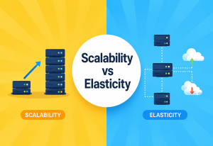
Because reads are served from a cache-fronted, purpose-built OLAP store, and Query Service instances are stateless, horizontal scaling is straightforward: add more instances behind the load balancer, add more OLAP store replica nodes, and grow the Redis cache tier as concurrent dashboard traffic increases. A well-tuned system can serve the large majority of dashboard queries with p99 latency in the tens of milliseconds, since the OLAP store’s columnar, pre-indexed design is built specifically for this query shape.
11.2 Scaling the ingestion path
The Stream Processor scales primarily by increasing Kafka topic partition count and running more parallel processing workers, since each partition can be consumed independently. Partitioning by seller ID means the system scales cleanly as seller count grows, at the cost of needing careful handling for a small number of unusually high-traffic sellers whose events might otherwise create a single overloaded partition; a common mitigation is sub-partitioning a small number of known high-volume sellers across multiple partitions specifically for their traffic.
11.3 Cost optimization
At this scale, both compute and storage cost are real constraints. Multi-granularity rollups, computed and stored at minute, hour, and day resolution, let the system serve any requested time range efficiently, but storing every granularity for every seller and product combination indefinitely adds up quickly; most systems apply a retention and downsampling policy, keeping fine-grained minute-level rollups for a short window, such as the last seven days, and only coarser hour or day rollups beyond that, since dashboards rarely need minute-level precision for data from months ago. Similarly, tuning the Redis cache TTL to just long enough to absorb repeated identical queries, without unnecessarily holding memory for rarely-repeated ones, keeps cache infrastructure cost proportional to actual traffic patterns rather than growing unboundedly with seller count.
11.4 Capacity planning example
As a concrete illustration, consider a marketplace with two million active sellers and a combined clickstream and order event volume of two hundred thousand events per second at peak. A well-partitioned Kafka cluster and Stream Processor fleet can comfortably sustain this volume with sub-minute end-to-end latency from raw event to updated rollup, given adequate partition count and processing parallelism, whereas attempting to achieve the same freshness by running frequent batch jobs against a general-purpose database, instead of a genuine streaming pipeline, would require infeasibly frequent batch cycles to approach the same latency, at far greater compute cost for a strictly worse result.
“A handful of extremely high-traffic sellers generate a disproportionate share of all events. How does that affect your partitioning strategy?” This is the classic hot-key problem in a partitioned streaming system. Partitioning purely by seller ID risks a small number of partitions becoming overloaded by these high-traffic sellers specifically. The mitigation is detecting known high-volume sellers and sub-partitioning their event stream across multiple partitions, using a composite key such as seller ID plus a hash bucket, then merging their partial aggregates back together at the Aggregation Service layer before writing the final rollup.
High Availability & Reliability
Sellers rely on this system for real business decisions — spotting a conversion drop during a live promotion, confirming a flash sale is performing as expected — which makes reliability a genuine product concern, not just an engineering one.
12.1 Redundancy at every layer
Every component — API Gateway, Load Balancer, Query Service instances, WebSocket Gateway, Redis, and the OLAP store — runs as multiple redundant nodes spread across at least three availability zones, so no single machine or zone failure takes dashboard availability down.
12.2 Graceful degradation
If the real-time OLAP store or Stream Processor becomes degraded, the Query Service falls back to the most recent cached results with a clear staleness indicator, rather than failing the dashboard outright, exactly as described in the storage section. This graceful degradation, paired with the circuit breaker pattern, is what keeps a temporary pipeline slowdown from becoming a visible outage for sellers.
12.3 Failure recovery in the streaming pipeline
If a Stream Processor worker crashes mid-window, Kafka’s committed consumer offsets mean the replacement worker resumes exactly where processing left off, and the idempotent, mergeable rollup-write pattern described earlier ensures reprocessing any in-flight events produces the same final result as if no crash had occurred.
12.4 Data durability and backup
The raw event log itself, retained in Kafka and the data warehouse, is the ultimate source of truth this system can always recompute from if a downstream store is ever corrupted or lost; OLAP store rollups are, in a real sense, a rebuildable cache over that durable event log rather than the sole copy of the data. This property is what makes the batch layer’s periodic full reconciliation both possible and trustworthy.
12.5 Chaos testing
Teams operating this kind of system at scale routinely inject failures deliberately — killing a Stream Processor worker mid-window, simulating an OLAP store node failure, forcing a Kafka broker restart during peak load — specifically to confirm that the fallback, circuit-breaker, and recovery mechanisms described in this section behave as designed under real conditions rather than only in theory.
The raw event log acting as the ultimate source of truth is like a bank’s transaction ledger. Even if a teller’s daily summary sheet gets lost or miscalculated, the full ledger can always be replayed to reconstruct the correct balance from scratch.
Security
Because this system exposes sensitive business data — sales figures, traffic, conversion rates — directly to independent third-party sellers who share the same underlying infrastructure, tenant isolation is as much a security concern here as it is a performance one.
- Strict tenant isolation at the query layer — every dashboard query is scoped to the authenticated seller’s own ID at the database and query-construction level, not just filtered in application code after the fact, so a bug in one layer cannot alone expose cross-seller data.
- Authentication and authorization — every dashboard request requires a valid seller session token, and the API Gateway verifies that the authenticated identity matches the seller ID being requested before the query ever reaches the Query Service.
- Rate limiting per seller — protects the platform from any single seller’s dashboard, automated tooling, or a misbehaving integration from generating disproportionate query load that could degrade the experience for others.
- Encryption in transit and at rest — standard TLS for all API and WebSocket traffic, and encryption at rest for the OLAP store and data warehouse, given the commercially sensitive nature of seller sales data.
- Audit logging on data access — access to seller analytics data, especially any internal tooling that can query across sellers for support or fraud investigation purposes, is logged for accountability given the sensitivity of the underlying business data.
Enforcing tenant isolation only in the Query Service’s application code, with no corresponding boundary at the storage layer itself. A single missed filter in one code path can then expose cross-seller data; partitioning and query construction at the storage layer should make that class of bug structurally much harder to introduce in the first place.
“How would you guarantee, at an architectural level, that seller A can never see seller B’s data, even if there’s a bug in the dashboard’s query-building code?” A strong answer points to storage-layer partitioning by seller ID combined with a query construction layer that always injects the authenticated seller’s ID as a mandatory filter before a query can even be built, ideally enforced by a shared internal library every service is required to use rather than something each service implements independently, so the isolation guarantee does not depend on every engineer remembering to add the filter correctly every time.
Monitoring, Logging & Metrics
14.1 Key metrics to track
| Metric | Why it matters |
|---|---|
| Dashboard query latency (p50, p95, p99) | Directly affects seller-perceived dashboard responsiveness |
| End-to-end event-to-dashboard latency | Measures how “real-time” the system actually is in practice |
| Kafka consumer lag | Rising lag means the aggregation pipeline is falling behind real time |
| Cache hit ratio | Low hit ratio signals rising OLAP store load ahead of time |
| Batch reconciliation delta | Large deltas between speed-layer and batch-layer results indicate a pipeline bug |
| WebSocket connection count and churn | Signals load on the WebSocket Gateway and potential client-side issues |
14.2 Logging and tracing
Every rollup write logs the inputs that produced it — which raw events contributed, which window they were assigned to, and whether the write was an initial finalization or a later correction — which is essential for debugging a specific seller’s reported discrepancy. Distributed tracing ties a single event’s journey together across Kafka, the Stream Processor, the Aggregation Service, and the OLAP store, which is invaluable when diagnosing why a specific metric took longer than expected to appear on a seller’s dashboard.
14.3 A typical debugging workflow
When a seller reports “my sales dashboard looks wrong,” the on-call engineer’s first step is comparing the speed-layer rollup for the relevant time bucket against the batch layer’s most recent reconciled value for the same bucket. If they match, the discrepancy is likely a seller misunderstanding of what a given metric actually measures, worth a support explanation rather than an engineering fix. If they diverge significantly, the next step is tracing a specific order or event through the pipeline using its event ID, checking whether it was correctly partitioned, windowed, and aggregated at each stage, which usually narrows the root cause to one specific service quickly.
Monitoring this system is like a factory’s quality control station comparing a fast in-line sensor reading against a slower, more thorough lab test on the same batch — most of the time they agree closely, and the rare cases where they diverge are exactly the signal worth investigating.
Deployment & Cloud
Modern real-time analytics systems are typically deployed on containers orchestrated by Kubernetes across multiple availability zones on a major cloud provider, often supplemented by managed streaming and analytical-database offerings given the specialized operational expertise those systems require.
- Canary releases for aggregation logic changes — a change to how a metric is computed is rolled out to a small percentage of sellers first, with close monitoring of reconciliation deltas, before a full rollout, since a subtle aggregation bug could otherwise silently mis-report sales figures for every seller at once.
- Blue-green deployment for the Query Service — a full parallel environment is stood up and traffic switched over only once health checks pass, allowing instant rollback.
- Infrastructure as code — Kubernetes manifests, Kafka topic configuration, and OLAP store cluster sizing are defined declaratively so environments are reproducible and auditable.
- Managed services where they reduce operational risk — many teams choose a managed Kafka offering and a managed real-time OLAP database rather than operating these highly specialized systems themselves, trading some cost for significantly reduced operational burden.
15.1 Testing and validation before release
Because a bug in aggregation logic could silently misreport real revenue figures to real sellers, changes to the Stream Processor or Aggregation Service are validated by replaying a recorded sample of real historical events through the new logic in a staging environment and comparing the output against known-correct historical rollups, and further validated through a shadow deployment that processes live production events in parallel with the current logic, writing to a separate, non-customer-facing table for comparison before any change is promoted to a canary rollout.

15.2 Multi-region operation
A marketplace operating across several regions typically deploys a full regional copy of the ingestion and OLAP layers, keeping each region’s sellers and their data served from infrastructure physically close to them, with only lightweight cross-region aggregation for any global reporting leadership might need, rather than routing every seller’s dashboard query across a long-haul network path to a single global deployment.
Advantages, Disadvantages & Trade-offs
Live Actionable Visibility
Gives sellers immediate, actionable visibility into their own performance, enabling faster reactions to promotions, issues, and trends than any batch reporting system could support.
Architectural Complexity
Adds substantial architectural complexity compared to simple batch reporting, and requires ongoing operational expertise in stream processing and specialized analytical databases.
Speed vs Exactness
The real-time speed layer trades a small, bounded amount of precision and completeness for dramatically lower latency compared to a fully exact batch computation.
16.1 Freshness versus availability
Another trade-off worth naming directly is the same consistency-versus-availability tension seen throughout distributed systems, here expressed as freshness versus availability. When the streaming pipeline falls behind during a traffic spike, the system can either block dashboard queries until it catches up, or serve the most recently available rollups with a visible staleness indicator. Nearly every production system in this space chooses availability, since a seller seeing slightly delayed numbers during a spike is a far smaller problem than a seller seeing no dashboard at all during exactly the high-traffic moment they most want visibility into their performance.
16.2 Granularity versus cost
A further trade-off exists between metric granularity and system cost. Offering every seller minute-level breakdowns by product, by traffic source, and by geography simultaneously sounds appealing, but the combinatorial growth in stored rollup rows across millions of sellers makes storing every possible dimension combination at the finest granularity prohibitively expensive. Most systems instead offer fine granularity only on the most commonly requested dimension combinations, with coarser granularity or on-demand computation for rarer combinations, which is a deliberate product and cost decision as much as a technical one.
16.3 Transparency versus simplicity in approximate metrics
A final trade-off worth naming is transparency versus simplicity in how approximate metrics are presented. Showing sellers an explicit confidence interval or error margin on every approximate metric is the most honest option, but it can also be confusing or overwhelming for sellers who simply want a quick number to glance at. Most production dashboards instead choose simplicity by default, presenting a single clean number, while quietly ensuring the underlying error bounds are small enough not to materially mislead typical business decisions, reserving explicit uncertainty indicators for cases where the approximation error could genuinely change what action a seller would take.
Best Practices & Common Mistakes
17.1 Best practices
- Always communicate to sellers, clearly and visibly, whether a given number on their dashboard is live speed-layer data or fully reconciled batch-layer data.
- Design tenant isolation into the storage and query-construction layers directly, not only as an application-level filter that depends on every code path remembering to apply it.
- Use approximate algorithms like HyperLogLog and count-min sketches deliberately and explicitly for metrics that can tolerate a small, bounded error, rather than either forcing exact computation everywhere or using approximation carelessly where exactness actually matters.
- Retain the full raw event log as the ultimate source of truth, treating every downstream rollup store as rebuildable from it rather than as the only copy of the data.
- Validate every change to aggregation logic against historical replay and shadow deployment before it ever reaches real seller-facing numbers.
17.2 Common mistakes
- Running live aggregation queries against raw transactional data instead of precomputed rollups, which is the naive approach that collapses under real scale.
- Broadcasting every metric update to every open WebSocket connection rather than using a targeted, per-seller subscription model.
- Silently blending real-time and reconciled figures without any staleness or freshness indicator, undermining seller trust the first time a number visibly changes after the fact.
- Storing every possible metric-dimension combination at the finest granularity for every seller regardless of actual usage, driving storage cost far beyond what the product actually needs.
- Skipping chaos and failure-injection testing for the streaming pipeline specifically, given how central its correct recovery behavior is to the entire system’s trustworthiness.
17.3 A pre-launch checklist
Before this system goes live for a meaningful share of real sellers, it is worth confirming each of the following explicitly: tenant isolation is enforced at the storage and query-construction layer, not just in application code; the batch layer’s reconciliation job is running on a known schedule with alerting on large deltas against the speed layer; approximate-metric error bounds have been validated against real traffic patterns; the WebSocket Gateway’s subscription model has been load tested at expected peak concurrent-connection counts; and dashboards for pipeline health, listed in the monitoring section, are wired up to alerting before real sellers depend on this data for business decisions.
Real-World Industry Examples
Large Marketplaces
Major online marketplaces that support large numbers of independent third-party sellers invest heavily in exactly this kind of real-time seller analytics, since seller trust and continued engagement with the platform depend directly on sellers being able to see, quickly and reliably, how their listings are actually performing.
Advertising Platforms
Digital advertising platforms solve a closely related problem for advertisers rather than sellers, showing live spend, impressions, click-through rate, and conversion metrics for active ad campaigns, using very similar underlying architecture — a streaming ingestion pipeline, a purpose-built real-time OLAP store, and a Lambda-style reconciliation process against exact billing data computed later.
Ride-Hailing & Delivery Driver Dashboards
Platforms with a large base of independent drivers or delivery couriers build a close cousin of this system for driver-facing earnings and performance dashboards, tracking completed trips, active hours, and earnings in near real time, with the same tenant-isolation and speed-versus-accuracy considerations applying directly, just with drivers in place of sellers as the “tenant” whose data must stay isolated and current.
Product Analytics Platforms
Dedicated product-analytics companies offer this exact category of system as a service to other businesses, letting a company embed live usage dashboards into their own product without building the underlying streaming and OLAP infrastructure themselves. These platforms are, architecturally, a direct real-world instance of the Lambda-architecture pattern described throughout this guide, packaged as a general-purpose product rather than built specifically for one marketplace’s sellers.
Trading & Portfolio Dashboards
Brokerage and trading platforms build a related category of real-time dashboard, showing live portfolio value, open position performance, and market data updates. The core architectural shape is similar — streaming market and trade events, a fast aggregation layer, and a push-based update mechanism to open dashboards — though financial contexts typically demand tighter accuracy guarantees than a marketplace sales dashboard, since even a small approximation error in a displayed price or balance can carry real regulatory and trust implications, which is why financial dashboards more often lean toward exact computation over approximate algorithms even at higher infrastructure cost.
“How would this design change for a driver-earnings dashboard on a ride-hailing platform instead of a seller-sales dashboard on a marketplace?” The core architecture transfers almost directly — completed trips replace completed orders, active-hours events replace clickstream, and drivers replace sellers as the isolated tenant — but the alerting and freshness expectations often need to be tighter, since a driver actively working right now cares about near-instant earnings feedback in a way that is closer to the alerting system’s sliding-window use case than to a seller casually checking sales once every hour.
Frequently Asked Questions
Why not just make everything exact and skip the approximate speed layer entirely?
Computing perfectly exact aggregates over a continuously growing, extremely high-cardinality dataset within a few seconds, for every possible query shape a seller might request, is not practically achievable at real marketplace scale without either enormous, cost-prohibitive infrastructure or accepting much higher latency than “real time” implies. The Lambda architecture’s approximate-then-reconciled approach is a deliberate, well-understood engineering trade-off, not a shortcut taken out of laziness.
How stale can speed-layer data actually get before it is a real problem?
Under normal operation, end-to-end latency from a raw event to an updated dashboard rollup is typically measured in seconds, well within what most sellers would consider “real time.” The threshold for genuine concern is when consumer lag or processing delay grows large enough that a seller could plausibly notice — commonly somewhere in the range of a minute or more sustained — which is exactly why lag-based alerting, described in the monitoring section, is tuned to catch this well before it becomes seller-visible.
Should every seller get identical dashboard features regardless of size?
Many marketplaces intentionally tier dashboard capabilities — offering finer time granularity, longer historical retention, or more detailed dimension breakdowns to larger or paying sellers — which is as much a product and cost decision as a technical one, but it does map cleanly onto the architecture described here, since the underlying rollup granularity and retention policy can be applied selectively per seller tier rather than uniformly across the entire marketplace.
Can a smaller marketplace build a simplified version of this system?
Yes. A marketplace with a modest seller count and event volume can start with a much simpler design — a scheduled job that recomputes aggregates every few minutes from the operational database into a small, dedicated reporting table, with no streaming pipeline at all. The full Lambda-architecture, stream-processing design in this guide becomes necessary primarily once seller count, event volume, and freshness expectations grow enough that periodic batch recomputation can no longer keep up.
How does this system avoid becoming a bottleneck for the checkout and storefront systems that produce its data?
By design, this system only ever consumes events published to Kafka; it never queries the operational order or storefront databases directly, and producing an event to Kafka is a fast, asynchronous, fire-and-forget operation from the storefront’s perspective. This decoupling is precisely what prevents any slowdown or failure in the analytics pipeline from ever propagating back and affecting checkout or browsing reliability.
Can sellers define their own custom metrics, or only choose from a fixed set?
Most production systems start with a fixed, well-understood set of core metrics — sales, sessions, conversion rate, and similar — computed centrally and efficiently through the rollup pipeline described throughout this guide, since predefined metrics are far cheaper to compute at scale than arbitrary ad hoc aggregations. Some platforms do eventually offer a limited custom-metric capability, typically implemented as a separate, more constrained query path against the batch layer’s data warehouse rather than the real-time speed layer, since arbitrary seller-defined aggregations are much harder to pre-compute efficiently and generally cannot meet the same real-time freshness guarantees as the core metric set.
Glossary
A quick-reference glossary of terms used throughout this guide, useful for review or as an interview refresher.
| Term | Plain-language definition |
|---|---|
| Rollup | A pre-aggregated summary of raw events over a fixed time bucket. |
| Speed layer | The fast, approximate real-time portion of a Lambda-architecture pipeline. |
| Batch layer | The slower, exact portion of a Lambda-architecture pipeline that reconciles the speed layer. |
| Tenant isolation | The guarantee that one seller’s data and queries are never visible to another seller. |
| HyperLogLog | A probabilistic data structure for estimating unique counts using a small, fixed amount of memory. |
| Watermark | A heuristic marker indicating a stream processor believes it has seen all events up to a point in time. |
| OLAP store | A database purpose-built for fast aggregation and group-by queries over large datasets. |
| Consumer lag | How far behind a message queue consumer is from the latest message produced. |
| Circuit breaker | A pattern that stops calling a failing dependency temporarily, falling back to a safe default instead. |
| CQRS | Command Query Responsibility Segregation; separating write and read paths into distinct flows. |
Summary & Key Takeaways
- Real-time seller analytics dashboards turn a continuous, high-volume stream of clickstream and order events into fast, accurate, per-seller metrics using a Lambda-architecture pattern of a fast approximate speed layer and a slower exact batch layer.
- The architecture splits into an ingestion and aggregation path built on Kafka and a stream processor, and a fast, cache-fronted read path served from a purpose-built real-time OLAP store rather than the operational transactional database.
- An API Gateway and Load Balancer sit at the front door for dashboard traffic, while a dedicated WebSocket Gateway handles live push updates through a targeted, per-seller subscription model.
- Approximate algorithms such as HyperLogLog and count-min sketches let the system compute high-cardinality metrics like unique visitors and top products efficiently, trading a small, bounded error for dramatically lower memory and compute cost.
- Tenant isolation, enforced at the storage and query-construction layer rather than only in application code, is as much a security requirement as a performance one, given how much commercially sensitive data this system exposes directly to independent third parties.
- Reliability patterns — circuit breakers, graceful degradation with clear staleness indicators, multi-zone redundancy, and a durable, replayable raw event log as the ultimate source of truth — matter enormously given how directly sellers rely on this data for real business decisions.
- The same underlying Lambda-architecture pattern, with different event sources and canonical metrics, generalizes directly to advertising campaign dashboards, driver-earnings dashboards, and general-purpose product-analytics platforms.
21.1 The one idea to remember
If you take away one idea from this entire guide, let it be this: a real-time seller analytics dashboard is fundamentally a Lambda-architecture problem wearing a marketplace-facing UI. Raw events land on a durable log; a streaming pipeline turns them into fast, approximate rollups the seller can see within seconds; a batch pipeline periodically reconciles those rollups against exact truth; and the whole thing is served through a cache-fronted, purpose-built OLAP store behind an API Gateway, a Load Balancer, and a targeted WebSocket push layer. Get those five pieces right — durable log, streaming rollups, batch reconciliation, OLAP-backed reads, and honest freshness communication — and everything else in this guide is either a variation on those themes or an operational detail supporting them.