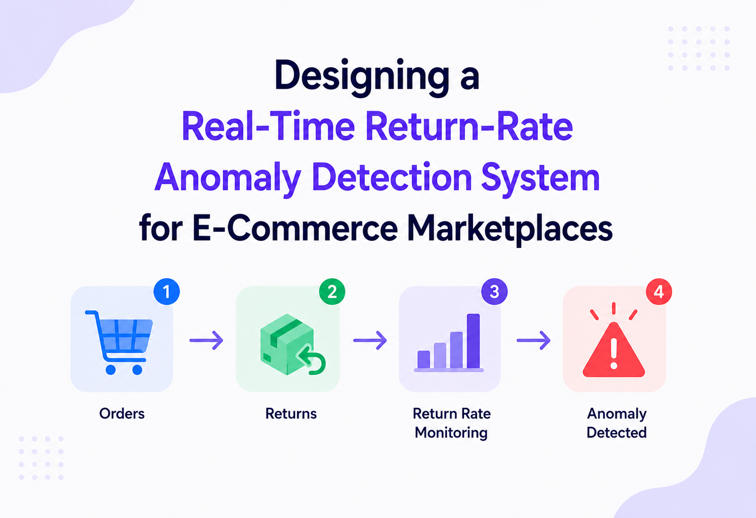
Designing a Real-Time Return-Rate Anomaly Detection System
How marketplaces detect, within one to two minutes, that returns for a category are behaving statistically abnormally — at a scale of millions of order and return events per minute, with z-score, EWMA, and CUSUM working together.
Introduction and History
A modern online marketplace is a giant department store with millions of aisles that never closes, restocks itself every second, and has no human standing at the returns counter to notice patterns. This chapter frames why detecting return-rate anomalies is one of the most important — and least visible — problems in e-commerce.
Every day, millions of packages go out, and — inevitably — thousands come back. Most of those returns are perfectly normal: a shirt didn’t fit, a gift was unwanted, a customer changed their mind. But sometimes returns spike for a reason that is NOT normal: a supplier shipped a defective batch of headphones, a seller’s product photos show the wrong color, a listing’s size chart is wrong, or a firmware update bricked a whole line of smart plugs.
In the early days of e-commerce, return rates were reviewed the way a shopkeeper reviews receipts: manually, weekly, by a merchandising analyst staring at a spreadsheet. That worked when a company sold thousands of products. It completely falls apart when a marketplace sells hundreds of millions of products across tens of thousands of categories, with new listings appearing every minute. By the time a human analyst notices a return-rate spreadsheet anomaly on a Friday, a defective product may have already been bought — and returned — by fifty thousand more customers.
This is why large marketplaces (Amazon, eBay, Walmart, Alibaba, Flipkart, Shopify-powered stores) invested heavily in building automated, real-time anomaly detection systems specifically for returns. Instead of asking “did this one order get returned?”, the system asks a much more powerful question: “Is the RATE of returns for this entire product category behaving abnormally, compared to its own history and to similar categories?” That shift — from single-event monitoring to statistical, category-level, real-time monitoring — is the heart of this tutorial.
By the end of this tutorial you will be able to answer, in interview-level depth, questions like: how do you ingest and process millions of order and return events per minute without losing any of them; how do you decide, mathematically, whether today’s return rate for a category is “just noise” or “a real problem”; how do you keep that decision fast (seconds to a couple of minutes) while also keeping it eventually accurate (accounting for returns that trickle in over weeks); and how do you build all of this so it keeps running correctly even when individual machines, availability zones, or entire regions fail. Along the way, every architectural box is explicitly labeled — API Gateway, Load Balancer, Message Broker, Stream Processing Cluster, and so on — so the diagrams read exactly like something you would draw on a whiteboard in a real system design interview.
1.1 A Short History of the Problem
Return-rate monitoring evolved through roughly four eras:
- 1Era 1 — Manual Reports (1990s–2000s): Weekly or monthly Excel-based reports generated by data analysts, reviewed by category managers. Detection lag: days to weeks.
- 2Era 2 — Batch ETL Dashboards (2000s–2010s): Nightly batch jobs (often Hadoop/Hive) computed return rates per category and displayed them on BI dashboards (Tableau, Looker). Detection lag: hours to a day.
- 3Era 3 — Streaming Analytics (2010s): With the rise of Apache Kafka, Apache Flink, and Spark Streaming, companies began computing rolling return rates in near real time. Detection lag: minutes.
- 4Era 4 — Real-Time Statistical Anomaly Detection (today): Modern systems combine streaming pipelines with statistical models (z-scores, EWMA, CUSUM) and even machine learning (isolation forests, seasonal-trend decomposition) to detect subtle anomalies within seconds to a couple of minutes, at the scale of millions of events per minute, with automatic alerting and even automatic mitigation (like temporarily suppressing a listing).
This tutorial designs an Era-4 system from scratch, assuming marketplace scale: millions of order and return events per minute, tens of thousands of categories, and a requirement to detect a real anomaly within one to two minutes of it starting.
“Why not just query the database every hour and compute return rate per category?” A strong answer explains that hourly batch queries introduce detection lag of up to an hour, during which thousands of defective units can ship, and that a proper design should support both a fast streaming path (seconds-to-minutes detection) and a slower, more accurate batch path (for auditing and model retraining) — the classic Lambda architecture trade-off, discussed later in this tutorial.
1.2 Batch vs. Streaming: A Direct Comparison
| Dimension | Nightly Batch Job | Real-Time Streaming (This Design) |
|---|---|---|
| Detection latency | Hours to a day | Under two minutes |
| Infrastructure complexity | Low — a scheduled SQL/Spark job | Higher — Kafka, Flink, stateful processing, alerting |
| Accuracy of final numbers | High — full data available | Approximate — early estimate, corrected later by batch reconciliation |
| Operational cost | Low | Higher — 24/7 cluster operation, on-call for the pipeline itself |
| Best suited for | Low-risk categories, exploratory analytics, model training | High-risk, fast-moving categories where hours of delay cause real customer harm |
The recommended design in this tutorial is not “streaming instead of batch” but “streaming AND batch,” each doing the job it’s best at — this is precisely why the Lambda architecture pattern recurs throughout large-scale marketplace systems.
Problem and Motivation
“Detect unusual returns” is too vague to design against. Let’s define the problem precisely.
2.1 Problem Statement
Design a system that continuously ingests two event streams — order events and return events — for a marketplace processing on the order of a million or more requests per minute, and that, for every product category (e.g., “Wireless Earbuds”, “Men’s Running Shoes”, “Baby Monitors”), computes a rolling return rate and determines whether that rate is statistically abnormal compared to:
- That category’s own recent historical baseline (e.g., last 30 days, same day-of-week/hour-of-day).
- Sibling categories in the same parent category (to rule out marketplace-wide events like a holiday return surge).
- Expected seasonal patterns (e.g., returns always spike the week after Christmas — that is NOT an anomaly).
When an anomaly is detected, the system must alert the right teams (trust & safety, category management, supply chain, seller operations) within one to two minutes, with enough context (which SKUs, which sellers, what reason codes) to start an investigation immediately — and ideally trigger automated mitigations such as temporarily flagging a listing for review.
2.2 Why This Is Hard
| Challenge | Why It’s Hard |
|---|---|
| Scale | A large marketplace generates millions of order/return events per minute across peak sale events (Black Friday, Prime Day). The pipeline must not fall behind. |
| Category cardinality | Tens of thousands of categories, each needing its own rolling statistics, updated continuously — this is a “many small time series” problem, not one big number. |
| Low base rates | Return rates are usually small (2%–15%). Small absolute changes can be statistically significant, and naive thresholds (“alert if returns > 20%”) miss subtle but real problems in categories whose normal rate is only 3%. |
| Seasonality & noise | Return rates naturally fluctuate by day of week, month, and promotional calendar. The system must separate real anomalies from expected fluctuation. |
| Delayed returns | A return can happen up to 30–90 days after purchase. The “denominator” (orders) and “numerator” (returns) are not aligned in time, which complicates rate computation. |
| Actionability | Detecting an anomaly is useless if it isn’t paired with enough context (top SKUs, sellers, reason codes, geographic clustering) for a human or automated system to act on it. |
A very common beginner mistake is to alert on absolute return counts instead of return rates. If a category simply sells more units on a given day (e.g., a flash sale), its return count will naturally rise even if the underlying return rate (returns ÷ orders) stays perfectly normal. Always normalize by volume before comparing to a baseline.
2.3 Goals
- Functional: near real-time (P95 < 2 minutes) category-level return-rate anomaly detection, with severity scoring and drill-down context.
- Non-functional: horizontal scalability to millions of events/minute, at-least-once delivery with idempotent processing, 99.95%+ availability, sub-second p99 read latency on the serving API, and strong observability.
2.4 Non-Goals
It’s equally important to state what this system is explicitly not trying to solve, since a clear boundary keeps the design focused. This system is not a general-purpose fraud-detection engine (it doesn’t try to catch an individual bad actor gaming returns), not a customer-service ticketing system (it hands off to existing ticketing/paging tools rather than replacing them), and not a root-cause diagnosis engine in the deep sense — it surfaces strong correlational signals (a specific SKU or seller dominating the excess returns) but leaves final root-cause confirmation (e.g., actually inspecting a returned unit) to a human investigator or a downstream quality process.
Core Concepts You Need First
Before drawing boxes and arrows, let’s build a shared vocabulary. Every term below is explained as if you have never heard it before.
3.1 Return Rate
What: The fraction of orders in a category that are eventually returned, over a given time window. Why: It’s the fundamental “health signal” for a category — a rising return rate usually means something is wrong with the product, the listing, or the shipping experience. Analogy: Like a restaurant’s “sent-back plates” rate — if 1 in 100 plates comes back to the kitchen, that’s normal; if 1 in 5 comes back tonight, the chef needs to know right now. Example: If “Wireless Earbuds” category had 10,000 orders and 400 confirmed returns in the trailing 24 hours, the return rate is 4%.
3.2 Event Stream
What: A continuous, ordered sequence of small messages (events) representing things happening in the system — an order placed, a return initiated. Why: Marketplaces are inherently event-driven; nothing waits for a nightly batch job anymore. Analogy: Like a news ticker at the bottom of a TV screen — new headlines (events) keep scrolling in, and anyone watching can react instantly. Example: Apache Kafka topics order-events and return-events.
3.3 Sliding Window Aggregation
What: Continuously computing an aggregate (like a count or rate) over a moving time range, e.g., “the last 15 minutes,” recalculated as time moves forward. Why: We need up-to-date rates without recomputing from all historical data every time. Analogy: A car’s average speed over the “last 5 minutes” gauge — it forgets old data as it slides forward. Example: A tumbling 1-minute window counts orders and returns per category, and a sliding 60-minute window aggregates 60 of those tumbling windows for a smoother rate.
3.4 Baseline / Seasonal Model
What: A statistical model of what “normal” looks like for a category at a given time (hour of day, day of week, season). Why: Without a baseline, you cannot know if today’s number is abnormal. Analogy: A thermostat doesn’t just look at “is it 75°F” — it compares against what temperature it should be for this time of year. Example: “Kids’ Toys” baseline return rate is 6% in November but 9% in the first week of January (post-holiday returns) — both are “normal” for their respective periods.
3.5 Z-Score / Statistical Significance
What: A number telling you how many standard deviations a data point is from the baseline mean. Why: It converts “is this different?” into a precise, comparable number regardless of the category’s scale. Analogy: Like grading on a curve — a z-score tells you how unusual a student’s score is compared to the whole class’s typical spread, not just the raw number. Example: A z-score of 4.2 for a category’s return rate means it’s over four standard deviations above normal — extremely unlikely to be random noise.
3.6 EWMA (Exponentially Weighted Moving Average)
What: A moving average that gives more weight to recent data points and exponentially less weight to older ones. Why: It reacts faster to real changes than a plain average while still smoothing out noise. Analogy: Like judging someone’s mood by their last few interactions, weighting the most recent one heaviest, rather than every interaction you’ve ever had with them equally. Example: Used to track a category’s “current” return rate that adapts quickly to genuine shifts.
3.7 CUSUM (Cumulative Sum Control Chart)
What: A technique that accumulates small deviations from a baseline over time to detect a sustained (even if small) shift, not just a single spike. Why: Some quality problems show up as a slow, steady creep rather than a sudden spike, and CUSUM catches that. Analogy: Like a scale that doesn’t care about one heavy meal but flags a slow, steady weight gain trend over weeks. Example: A CUSUM chart flags when a category’s return rate has been creeping up by 0.3% every hour for six hours straight.
3.8 Idempotency
What: A property where processing the same event multiple times produces the same result as processing it once. Why: Distributed systems retry messages; without idempotency, a retried “return” event could be double-counted. Analogy: Pressing an elevator button that’s already lit doesn’t call two elevators. Example: Using the unique return_id as a deduplication key in the stream processor’s state store.
3.9 Backpressure
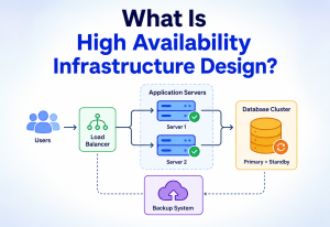
What: A flow-control mechanism where a slow downstream component signals upstream components to slow down, instead of being overwhelmed. Why: At a million-plus events per minute, without backpressure a slow consumer causes unbounded queue growth and eventual crash. Analogy: A highway on-ramp traffic light that only lets cars merge when there’s room downstream. Example: Kafka consumer lag triggers autoscaling of stream-processing workers.
3.10 Partitioning & Consistent Hashing
What: Splitting a large stream or dataset into smaller, independently processed pieces (partitions), typically assigned by hashing a key such as category_id. Why: No single machine can process a million-plus events per minute; partitioning is what lets many machines share the work while still guaranteeing that all events for the same category are processed in order, by the same worker, so per-category counters stay correct. Analogy: A large post office sorting mail into hundreds of bins by zip code so that no single sorter has to touch every letter, yet all mail for one zip code always ends up together. Example: The return-events Kafka topic uses 300 partitions, with a custom partitioner hashing category_id (and further salting a handful of extremely high-volume categories to prevent a single partition from becoming a bottleneck).
3.11 CAP Theorem (Applied Here)
What: A distributed systems principle stating that under a network partition, a system must choose between Consistency (every read sees the latest write) and Availability (every request gets a response, even if possibly stale). Why: It forces an explicit, honest choice rather than an accidental one. Analogy: Two people updating the same shared shopping list from different rooms during a power outage in the connecting hallway — they can either stop writing until the connection is restored (consistency) or keep writing on their own copies and reconcile later (availability). Example: This system deliberately chooses availability and eventual consistency for the fast streaming path — a dashboard might show a rate that’s a few seconds stale — because a returns-monitoring system should never stop accepting return events just to guarantee perfectly fresh reads.
3.12 Replication
What: Keeping multiple copies of the same data (a Kafka partition, a Redis shard) on different machines. Why: If one machine dies, a replica already has the data, so no event or counter is lost. Analogy: Keeping a spare key with a trusted neighbor in case you lose yours. Example: Kafka topics are configured with replication factor 3, so any single broker failure is invisible to producers and consumers.
Architecture and Components
Now let’s assemble these concepts into a full system. Every box below is deliberately labeled with its specific role (API Gateway, Load Balancer, etc.) so the diagram reads like a real production architecture — exactly what an interviewer expects to see on a whiteboard.
4.1 High-Level Architecture Diagram
4.2 Component Responsibilities
| Component | Responsibility |
|---|---|
| Client Apps (Web/Mobile/Seller Portal) | Sources of order placement and return-initiation actions. |
| Edge / CDN + WAF | TLS termination, DDoS protection, static asset caching, first line of defense. |
| API Gateway | Single entry point for all client requests; handles auth, rate limiting, request routing, and request/response transformation before forwarding to backend services. |
| Load Balancer (L4/L7) | Distributes incoming traffic across many stateless service instances; performs health checks and removes unhealthy nodes from rotation. |
| Order Service | Owns order lifecycle; emits OrderPlaced events. |
| Returns Service | Owns return-request lifecycle; emits ReturnInitiated/ReturnCompleted events. |
| Message Broker (Kafka) | Durable, partitioned, ordered event backbone decoupling producers from consumers; absorbs traffic bursts. |
| Stream Processing Cluster (Flink/Kafka Streams) | Consumes order & return streams, computes per-category rolling counts/rates in tumbling and sliding windows, performs stateful joins. |
| Anomaly Detection Engine | Applies statistical models (z-score, EWMA, CUSUM) plus seasonal baselines to each category’s computed rate stream to flag anomalies. |
| Baseline / Feature Store | Stores historical per-category seasonal baselines (mean, std-dev by hour/day) used by the detection engine. |
| Hot Store / Cache (Redis) | Low-latency store for current rolling counters and recent anomaly state, read by the serving API. |
| Time-Series Database (columnar OLAP) | Stores computed per-category-per-minute metrics durably for dashboards and historical queries. |
| Alerting & Notification Service | Converts detected anomalies into pages, emails, Slack messages, and tickets, applying de-duplication and severity routing. |
| Serving API + its own Gateway/LB | Read-optimized API for dashboards and internal tools to query current/historical category health, fronted by its own gateway and load balancer for isolation from ingestion traffic. |
| Data Lake (Batch Layer) | Raw event archive used for nightly re-computation, auditing, and model retraining — the “batch” half of the Lambda architecture. |
| Config / Rules Service | Stores per-category thresholds, suppression rules, and on-call routing, editable without redeploying the detection engine. |
“Why put an API Gateway and Load Balancer in front of BOTH the ingestion path and the serving/read path, instead of sharing one?” Answer: ingestion traffic (orders/returns) and read traffic (dashboards, internal tools querying anomaly status) have very different load profiles and failure domains. Isolating them means a dashboard-query storm from an internal tool cannot degrade the critical path that detects real product-quality issues, and vice versa. This is bulkhead isolation applied to the API layer.
4.3 Component Deep-Dive
What: A managed layer (e.g., Kong, Amazon API Gateway, Apigee) sitting in front of backend services. Why here: All order/return writes and all anomaly-status reads pass through a gateway so we get centralized authentication, per-client rate limiting, request validation, and observability without duplicating that logic in every microservice. Production example: Amazon’s internal service mesh uses gateway-like proxies in front of every customer-facing API to enforce quotas across thousands of internal teams.
What: A component (L4 network LB plus L7 HTTP LBs, or a service-mesh sidecar) that spreads requests across many identical service replicas. Why here: At a million-plus requests per minute, no single instance can handle traffic; the load balancer is what makes horizontal scaling actually work, and its health checks are what makes failover automatic.
What: A distributed, partitioned, replicated log. Why here: It decouples the Order/Returns services (producers) from the Stream Processing Cluster (consumers), so a slowdown in analytics never blocks a customer’s checkout, and it absorbs traffic spikes (like Black Friday) by simply growing its backlog instead of dropping data.
What: A distributed compute engine (Apache Flink is the industry standard for this exact use case) that maintains windowed, keyed state per category. Why here: This is where “count orders and returns per category per minute” actually happens continuously and in a fault-tolerant, exactly-once-semantics way via checkpointing.
What: A component — often implemented as another Flink job or a dedicated microservice consuming the aggregated-rate stream — that compares each category’s live rate against its baseline using statistical tests. Why here: Separating “compute the rate” from “decide if the rate is abnormal” lets each be scaled, tested, and evolved independently (e.g., swapping z-score for a machine-learned model later without touching the aggregation logic).
What: An in-memory key-value store. Why here: Dashboards and the serving API need sub-10ms reads of “what is category X’s return rate right now” — querying a time-series database or data lake directly for every dashboard refresh would be far too slow at this request volume.
What: A columnar database purpose-built for time-stamped metric queries (e.g., a ClickHouse-style engine). Why here: Historical trend queries (“show me this category’s return rate for the last 90 days”) need efficient range scans and aggregation that a row-oriented OLTP database handles poorly at this scale.
Internal Working (Step-by-Step)
Let’s trace what happens the moment a customer initiates a return.
- The customer clicks “Return this item.” The mobile app hits the Ingestion API Gateway, which is protected by CDN + WAF for TLS, DDoS defense, and geo-based edge routing.
- The API Gateway authenticates the request (OAuth token), applies rate limiting, then forwards to a Load Balancer, which round-robins to a healthy instance of the Returns Service.
- The Returns Service writes the return record to its own database and publishes a
ReturnInitiatedevent to the Kafka topicreturn-events, partitioned bycategory_id. This is done via the outbox pattern to guarantee that the DB write and the event publish either both succeed or neither does. - Kafka replicates the event to three brokers for durability. It is now safe from any single broker crash.
- A Flink Stream Processing Cluster consumes
return-events. Because the topic is partitioned bycategory_id, all events for a single category go to the same worker, whose per-category counters stay perfectly consistent and in order. - The Flink job maintains, per category, a rolling window: e.g., number of orders in the last 60 minutes (from
order-events) and number of returns in the last 60 minutes (fromreturn-events). Every 1-minute tumbling window emits the current rate. - The rate stream is fed into the Anomaly Detection Engine, which loads the seasonal baseline (mean μ and standard deviation σ) for “this category, this hour, this day of week” from the Feature Store and computes a z-score. If |z| > threshold, and the anomaly persists over multiple consecutive windows (to avoid single-spike false alarms), a signal is emitted onto the
anomaly-eventstopic. - The Alerting Service consumes
anomaly-events, de-duplicates against active incidents, and pages the on-call team with a link to a pre-built dashboard showing top contributing SKUs, sellers, and return reasons for that category.
A subtle but important detail: because returns can happen days or weeks after the original order, the streaming pipeline computes an early estimate of the return rate using the recent order and return activity. The batch layer later corrects this by joining every return with its original order (regardless of how old) and computing the true cohort-level return rate. Dashboards clearly label the two — “live rolling rate” vs. “finalized cohort rate” — so operators are never misled.
Data Flow and Lifecycle
Zooming out to see how a single anomaly moves through every layer of the system.
“What happens if the Alerting Service is down for 5 minutes?” Answer: because anomalies are published to a Kafka topic (anomaly-events), the messages are durably stored and simply queue up. When the Alerting Service recovers, it resumes consumption from its last committed offset, applies de-duplication (idempotency by anomaly_id), and pages responsibly — no anomaly is ever “lost” even though notifications are briefly delayed.
Anomaly Detection Algorithms In Depth
The heart of this system is deciding, mathematically, whether a number is “weird.” Let’s go through the techniques used together, each catching a different failure pattern.
1. Z-Score Against a Seasonal Baseline
What: Measures how many standard deviations the current return rate is from the expected mean for this specific hour-of-week. Why: Catches sudden, sharp spikes (e.g., a bad batch causing an immediate jump from 4% to 15%). Formula: z = (x − μ) / σ, where μ and σ are computed per category, per hour-of-day, per day-of-week, from a trailing 8–12 week window, refreshed nightly by the batch layer. Weakness: Needs enough historical volume per category to have a stable μ/σ — very low-traffic categories need a fallback (see below).
2. EWMA (Exponentially Weighted Moving Average) Control Chart
What: Tracks a smoothed “current” rate that reacts faster than a simple average but is still resistant to single-point noise. Why: Complements the z-score by being sensitive to a rate that’s climbing steadily minute over minute, even before it crosses the full z-score threshold. Formula: EWMA_t = α·x_t + (1−α)·EWMA_(t−1), with α typically 0.2–0.3 for minute-level data. An alert fires if EWMA exceeds μ + L·σ_EWMA for L≈2.7–3 (a standard EWMA control-chart constant).
3. CUSUM (Cumulative Sum)
What: Accumulates the signed deviation from baseline over time; resets to zero if it goes negative. Why: Best at catching small, sustained shifts that neither a single-window z-score nor EWMA would flag quickly (e.g., a slow quality-control drift at a factory). Formula: S_t = max(0, S_(t−1) + (x_t − μ − k)), alert when S_t > h (h is the decision threshold, k is an allowance/slack constant, typically 0.5σ).
4. Cold-Start / Low-Volume Fallback
What: For categories with too few orders to have a statistically stable baseline (e.g., a niche category with only 50 orders/day), the system falls back to a Bayesian approach — comparing against the sibling categories’ aggregated rate (borrowing statistical strength) instead of the category’s own thin history, using something like a Beta-Binomial model with a shrinkage estimator.
Formula (Beta-Binomial shrinkage): Model each category’s true return probability as drawn from a Beta(α, β) prior fitted from the parent category’s aggregate rate and variance. A category’s shrunken estimate is p_shrunk = (returns + α) / (orders + α + β). As the category’s own order volume grows, this estimate naturally converges to the category’s own empirical rate; when volume is tiny, it leans heavily on the parent category’s prior. This avoids two failure modes at once: a 2-order category showing “100% return rate” after a single unlucky return, and a 2-order category never triggering any anomaly at all because there’s technically “not enough data.”
5. Multi-Dimensional Drill-Down (Root-Causing an Anomaly)
What: Once a category-level anomaly fires, the system automatically decomposes the spike along secondary dimensions — SKU, seller, warehouse/fulfillment-center, geography, and return reason code — to surface the likely root cause instead of leaving a human to guess. Why: “Wireless Earbuds returns are up 3x” is an alert; “92% of the excess returns are SKU-88213 from Seller-4471, reason code DEFECTIVE_AUDIO” is an actionable ticket. How it works: The Anomaly Detection Engine, upon crossing threshold, issues a fast fan-out query against the same windowed state (or a secondary Flink job keyed by category+SKU+seller) to rank contributors by their share of the excess returns above baseline, attaching the top 3–5 contributors directly onto the AnomalyDetected event.
“How would you distinguish a single bad seller/SKU problem from a true category-wide issue (e.g., a new sizing standard confusing all buyers)?” Answer: by checking contributor concentration — if one SKU/seller accounts for the overwhelming majority (say, >70%) of the excess returns, it’s a targeted product/seller issue; if the excess is spread thinly and evenly across many SKUs/sellers in the category, it points to a category-wide cause (e.g., a listing-template change, a shared marketing claim, or a broader logistics problem).
Java: A Simplified Anomaly Scoring Component
// CategoryAnomalyScorer.java
// Applies z-score, EWMA, and CUSUM checks to a category's incoming rate sample.
public class CategoryAnomalyScorer {

    private final double alpha;          // EWMA smoothing factor
    private final double cusumSlackK;    // CUSUM allowance
    private final double cusumThresholdH;
    private final double zThreshold;

    private double ewma;
    private double cusum = 0.0;
    private boolean initialized = false;

    public CategoryAnomalyScorer(double alpha, double cusumSlackK,
                                  double cusumThresholdH, double zThreshold) {
        this.alpha = alpha;
        this.cusumSlackK = cusumSlackK;
        this.cusumThresholdH = cusumThresholdH;
        this.zThreshold = zThreshold;
    }

    /**
     * Evaluate one new minute-level return rate sample for a category.
     * baselineMean / baselineStdDev come from the seasonal Baseline Store,
     * keyed by (categoryId, hourOfDay, dayOfWeek).
     */
    public AnomalyResult evaluate(String categoryId, double currentRate,
                                   double baselineMean, double baselineStdDev) {

        if (!initialized) {
            ewma = currentRate;
            initialized = true;
        } else {
            ewma = alpha * currentRate + (1 - alpha) * ewma;
        }

        double safeStdDev = Math.max(baselineStdDev, 1e-6); // avoid divide-by-zero
        double zScore = (currentRate - baselineMean) / safeStdDev;

        double deviation = currentRate - baselineMean - cusumSlackK * safeStdDev;
        cusum = Math.max(0.0, cusum + deviation);

        boolean zAnomaly = Math.abs(zScore) > zThreshold;
        boolean ewmaAnomaly = Math.abs(ewma - baselineMean) > 2.7 * safeStdDev;
        boolean cusumAnomaly = cusum > cusumThresholdH;

        Severity severity = Severity.NONE;
        if (zAnomaly && cusumAnomaly) {
            severity = Severity.CRITICAL;
        } else if (zAnomaly || cusumAnomaly) {
            severity = Severity.HIGH;
        } else if (ewmaAnomaly) {
            severity = Severity.WATCH;
        }

        return new AnomalyResult(categoryId, currentRate, zScore, ewma, cusum, severity);
    }

    public enum Severity { NONE, WATCH, HIGH, CRITICAL }

    public record AnomalyResult(String categoryId, double currentRate, double zScore,
                                 double ewma, double cusum, Severity severity) {}
}Using a single global threshold (e.g., “z > 3 for every category”) sounds simple but breaks down because categories have wildly different volumes and natural variance — a high-volume category like phone cases may have a very tight, stable baseline, while a low-volume category like “vintage typewriters” naturally swings wildly day to day. Per-category, volume-aware thresholds (or the Bayesian shrinkage fallback above) are essential.
Advantages, Disadvantages & Trade-offs
Advantages
- Detects quality/listing problems within one to two minutes instead of days, drastically reducing the number of customers affected before a fix or listing suspension.
- Statistical, per-category baselines avoid both false alarms (during expected seasonal surges) and blind spots (in low-traffic categories, via the Bayesian fallback).
- Decoupled event-driven architecture means the detection pipeline never adds latency to the customer-facing checkout or returns flow.
- The same streaming infrastructure can be reused for other anomaly types (fraud spikes, delivery delay spikes) with minimal new plumbing.
- Automatic root-cause context (top SKUs, sellers, reason codes) shortens the time between “an alert fired” and “someone knows what to do about it,” which is often the more expensive half of an incident’s total cost.
- Because the pipeline is entirely event-driven, adding a new consumer (say, a future machine-learning model that wants the same order/return stream) requires zero changes to the existing Order/Returns services — it simply subscribes to the existing Kafka topics.
Disadvantages & Trade-offs
- Complexity vs. speed: A batch-only system (Era 2/3) is far simpler to build and operate but detects issues hours to a day late; the streaming + statistical approach trades operational complexity for speed.
- Return lag: Because a “true” return rate isn’t fully known until the return window closes (up to 30–90 days), the real-time rate is always an early estimate. The system must clearly label it as such and reconcile with the batch layer later.
- Cold-start categories: Brand-new categories or products have no baseline yet; the system must have an explicit bootstrapping strategy (e.g., borrow from parent category) or accept reduced sensitivity for the first few weeks.
- Alert fatigue risk: Overly sensitive thresholds create noisy pages that erode trust in the system; overly conservative thresholds miss real problems. Tuning is an ongoing operational cost, not a one-time task.
“Would you always choose the streaming approach over a simpler batch job?” A nuanced answer: no — if the business only needs daily insight (e.g., a small marketplace with low return-volume risk), a nightly batch job is far cheaper to build and run. The streaming architecture is justified specifically because return-rate anomalies at marketplace scale can cause large, fast-compounding financial and reputational damage if undetected for hours.
Performance & Scalability (Million-Requests-Per-Minute)
The problem calls out a scenario of millions of requests per minute. Let’s size the system for that.
9.1 Back-of-the-Envelope Estimation
- Assume 2 million order events/minute and 200,000 return events/minute at peak (a 10% return rate applied over a lagged window, though actual returns lag orders — this is a simplified peak-load estimate for the returns write path, not the true trailing rate).
- That is roughly 33,000 order events/sec and 3,300 return events/sec sustained at peak, with bursts 3–5× higher during flash sales.
- Each event is small (~300–500 bytes JSON or ~150 bytes Avro/Protobuf). At 33,000 events/sec × 500 bytes ≈ 16.5 MB/sec raw ingress for orders alone — trivial for Kafka, which routinely handles GB/sec clusters.
- Partition count: to parallelize across tens of thousands of categories without hot partitions, use a higher partition count (e.g., 200–500 partitions per topic) with a partitioner that hashes
category_id, and additionally salt extremely hot categories (like “Phone Cases”) to avoid partition skew.
9.2 Scaling Techniques Per Layer
| Layer | Scaling Technique |
|---|---|
| API Gateway / Load Balancer | Horizontally auto-scaled stateless instances behind a managed load balancer; scale on CPU + request-rate metrics; enable connection keep-alive and HTTP/2 to reduce connection overhead at high RPS. |
| Order/Returns Services | Stateless microservices, horizontally scaled; database writes go through connection pooling and, if needed, sharded by category or seller ID. |
| Kafka | Scale by adding brokers and partitions; use replication factor 3 for durability; tune acks=all for the returns topic (correctness-critical) and consider acks=1 for less critical telemetry. |
| Flink Cluster | Scale task managers horizontally; parallelism should match or exceed partition count; use RocksDB state backend with incremental checkpointing to keep large keyed state (per-category windows) manageable. |
| Redis Hot Store | Use Redis Cluster (sharded) keyed by category_id hash slot; read replicas for the dashboard read path. |
| Time-Series Store | Columnar, horizontally sharded store with time-based partitioning (e.g., daily partitions) for efficient range pruning. |
| Serving API | Cache-aside pattern in front of Redis/TSDB; CDN caching for largely-static dashboard assets. |
Amazon’s internal metrics pipelines are known to process tens of millions of events per second across all services combined, using Kafka-like durable logs and Flink-like stream processors with keyed, checkpointed state — the same architectural pattern described here, just at a larger aggregate scale spanning many pipelines.
9.3 Storage & State Sizing
- Kafka retention: Retaining 7 days of order/return events at ~16.5 MB/sec average ingress translates to roughly 10 TB of raw retained data per topic (before compression), which is comfortably handled by a modestly sized Kafka cluster using tiered/remote storage for older segments.
- Flink keyed state: With ~50,000 active categories, each holding a small rolling window struct (counts, EWMA, CUSUM accumulator — a few hundred bytes each), total keyed state is on the order of tens of megabytes, trivially small; the real scaling constraint is event throughput and checkpoint I/O, not state size.
- Redis hot store: ~50,000 categories × a few hundred bytes of current-state payload is only tens of megabytes — Redis is massively over-provisioned for data volume here and is sized instead for connection concurrency and read QPS from the dashboard/serving path.
- Time-series store: 50,000 categories × 1 row/minute × 1 year ≈ 26 billion rows; a columnar store with daily partitioning and category_id as a sort/index key keeps range-scan queries (“last 90 days for this category”) fast despite the volume.
9.4 Handling Traffic Spikes (Black Friday Style)
- Autoscaling policies pre-warmed ahead of known peak events (predictive scaling) rather than purely reactive scaling, since reactive scaling can lag a sudden 5× spike by minutes.
- Backpressure-aware consumers: Flink’s checkpoint-based backpressure naturally slows consumption rather than crashing under load; Kafka simply retains the backlog.
- Load shedding at the edge: If the ingestion path is truly saturated beyond provisioned capacity, shed the least-critical telemetry (e.g., non-critical UI analytics) before ever shedding order/return events.
High Availability & Reliability
- Multi-AZ deployment: Every stateful component (Kafka brokers, Flink task managers, Redis, the TSDB) is deployed across at least three availability zones, so a single zone failure never takes down the whole pipeline.
- Exactly-once / idempotent processing: Flink’s checkpointing plus idempotent sinks (keyed by
return_id/order_id) ensure that reprocessing after a failure doesn’t double-count events — critical since double-counted returns would produce false anomalies. - Graceful degradation: If the Anomaly Detection Engine is temporarily down, raw rolling rates still flow to the Time-Series store and dashboards, so humans retain visibility even without automated alerting (a form of fail-safe degradation rather than total blackout).
- Circuit breakers between the Serving API and its dependencies (Redis, TSDB) prevent a slow dependency from cascading into API-wide timeouts.
- Disaster recovery: Kafka topics replicated cross-region (e.g., via MirrorMaker2) for the returns topic specifically, since it’s the most business-critical stream; the Data Lake archive serves as the ultimate source of truth for full reprocessing if needed.
- Chaos testing: Regularly killing individual Flink task managers, Kafka brokers, and Redis nodes in a staging environment to verify that failover, checkpoint recovery, and consumer rebalancing behave as designed before a real outage tests them for the first time in production.
- Health checks and readiness probes: Every stateless service exposes liveness/readiness endpoints consumed by the load balancer and the orchestration layer, ensuring traffic is only routed to instances that are actually ready to serve, not just “running.”
10.1 Failure Scenarios Worked Through
| Failure | System Behavior |
|---|---|
| One Kafka broker crashes | Replication factor 3 means two other brokers already hold the data; producers/consumers reconnect to a surviving broker automatically with no data loss. |
| A Flink task manager crashes mid-window | The job restarts from the last successful checkpoint; because sinks are idempotent (keyed by event ID), replayed events don’t double-count. |
| Redis hot store becomes unavailable | The Serving API’s circuit breaker trips, falling back to reading directly from the Time-Series store with slightly higher latency rather than failing outright. |
| The Anomaly Detection Engine itself goes down | Rolling rates keep flowing into the Time-Series store and dashboards; humans lose automated alerting but retain full visibility, and the engine resumes from its last Kafka offset once restarted. |
| An entire availability zone fails | Multi-AZ deployment means load balancers route around the failed zone within health-check intervals (typically seconds), and stateful components (Kafka, Redis) already have in-sync replicas in the surviving zones. |
“What’s your RPO/RTO for this system if an entire region goes down?” A strong answer distinguishes: for the streaming/alerting path, an RTO of a few minutes and RPO of near-zero (thanks to replicated Kafka) is achievable; for full historical accuracy, the batch layer’s nightly reconciliation guarantees eventual RPO of zero because the Data Lake retains raw immutable events.
Security
- Authentication & Authorization: The API Gateway enforces OAuth2/JWT-based auth for both write (order/return) and read (dashboard) paths; internal service-to-service calls use mutual TLS (mTLS) within the service mesh.
- Data-in-transit encryption: TLS everywhere — client-to-gateway, gateway-to-service, service-to-Kafka (Kafka supports SASL_SSL).
- Data-at-rest encryption: Encrypted disks/volumes for Kafka logs, Redis persistence, and the Data Lake, with managed key rotation.
- PII minimization: Order/return events used by the anomaly pipeline should carry only category, SKU, seller, and reason-code fields — not raw customer PII — following data-minimization principles; a separate, access-controlled service handles customer-identifiable data if ever needed for an investigation.
- Rate limiting & abuse protection: The API Gateway enforces per-client and per-IP rate limits to prevent abusive scripted return submissions from skewing detection or overwhelming ingestion.
- Audit logging: Every configuration change to thresholds/rules (via the Config/Rules Service) is logged immutably, since a malicious or accidental threshold change could suppress real alerts.
Teams sometimes let internal dashboard tools query the production Redis hot-store or Kafka topics directly “for convenience.” This bypasses the API Gateway’s auth/rate-limiting and creates an invisible dependency that can silently break when internal schemas change. Always route even internal read traffic through a defined Serving API.
Monitoring, Logging & Metrics
A system whose entire job is “detect anomalies” must itself be relentlessly observable — you cannot trust a smoke detector you can’t verify is working.
12.1 Key Metrics to Track
| Metric | Why It Matters |
|---|---|
| End-to-end detection latency (order/return event → alert fired) | Directly measures whether the SLA (P95 < 2 min) is being met. |
| Kafka consumer lag (per topic/partition) | Early warning that the stream processor is falling behind — a leading indicator of detection-latency degradation. |
| Flink checkpoint duration & failure rate | Long or failing checkpoints threaten exactly-once guarantees and can stall processing. |
| Alert volume & false-positive rate (tracked via analyst feedback) | Guards against alert fatigue and validates threshold tuning. |
| Serving API p50/p95/p99 latency and error rate | Standard API health signals for the dashboard/read path. |
| Baseline staleness (age of last successful nightly baseline refresh) | A stale baseline silently degrades detection accuracy without any obvious error. |
12.2 Logging & Tracing
- Structured, correlation-ID-tagged logs across every service, so a single
return_idcan be traced from ingestion through aggregation to (possibly) an alert. - Distributed tracing (OpenTelemetry) spanning the API Gateway → service → Kafka → Flink → Alerting hops to pinpoint where latency accumulates.
- Dashboards (Grafana-style) showing per-category live return rate vs. baseline band, refreshed every minute, as the primary human-facing view.
- Sampled, structured logging for high-cardinality debug details (e.g., per-event trace logs) versus unsampled logging for anything tied to an alert firing, balancing storage cost against forensic completeness exactly where it matters most.
12.3 Alerting Metrics: Precision and Recall
Beyond system-health metrics, the detection logic itself needs its own quality metrics, tracked over time just like a machine-learning model would be: precision (of all alerts fired, what fraction were confirmed real issues by an analyst) and recall (of all known real issues, retrospectively, what fraction did the system actually catch, and how quickly). Tracking these two numbers over months is what turns threshold tuning from guesswork into an evidence-based process, and it’s usually the single most requested reporting metric from the trust-and-safety and category-management teams who consume these alerts daily.
eBay’s real-time analytics teams have publicly discussed using Kafka + stream processing with dedicated “pipeline health” dashboards separate from “business metric” dashboards — precisely because a healthy-looking business metric can hide an unhealthy pipeline that’s simply stale.
Deployment & Cloud
- Containerization: All stateless services (Order Service, Returns Service, Serving API, Alerting Service) packaged as containers, orchestrated via Kubernetes for self-healing and rolling deployments.
- Managed streaming infra: Kafka can be self-managed or a managed offering (e.g., a managed Kafka service); Flink can run on Kubernetes via a Flink Operator, or as a managed streaming analytics service.
- Infrastructure as Code: Terraform (or similar) defines the Kafka clusters, Kubernetes node pools, Redis clusters, and networking, enabling reproducible environments and safe disaster recovery rebuilds.
- CI/CD with canary releases: Changes to the Anomaly Detection Engine (e.g., a new statistical model) are deployed via canary — routing a small percentage of categories to the new logic and comparing detection outcomes against the old logic before a full rollout.
- Blue-green for the Serving API: Since it’s read-heavy and stateless, blue-green deployment gives instant rollback if a new version regresses latency.
- Environment parity: Staging mirrors production topology (same partition counts proportionally scaled down, same Flink parallelism ratios) so that load and latency behavior observed in staging is a reasonably faithful predictor of production behavior, rather than a much smaller setup that hides scaling issues until launch day.
Databases, Caching & Load Balancing
- Redis (cache/hot store): Holds the last 60–120 minutes of per-category counters and the latest anomaly status, with a TTL-based eviction for anything older, since the TSDB is the durable source of truth.
- Time-Series/OLAP store: Partitioned by day, indexed by category_id, storing per-minute aggregates for up to a year for trend analysis and model retraining.
- Transactional databases (Order/Returns services): Each owns its own database (database-per-service pattern) to avoid tight coupling; changes are propagated via the event stream (an outbox pattern ensures the DB write and the event publish are atomic).
- Load balancing strategy: L4 load balancing for raw TCP-level distribution across gateway instances, L7 (HTTP-aware) load balancing at the gateway for path-based routing and finer health checks; consistent hashing at the Kafka partitioner level to keep a category’s events on the same partition (and thus the same Flink sub-task) for stateful correctness.
“Why not just query the Order/Returns transactional databases directly for the return rate?” Because OLTP databases are optimized for point lookups and small transactional writes, not high-frequency aggregate scans across millions of rows per minute — doing so would either slow down the live checkout/returns systems or require expensive read replicas that still don’t scale to real-time streaming aggregation as cleanly as a purpose-built pipeline.
APIs & Microservices
15.1 Sample Serving API
GET /v1/categories/{categoryId}/return-rate?window=60m
Response 200:
{
  "categoryId": "electronics-wireless-earbuds",
  "windowMinutes": 60,
  "currentRate": 0.146,
  "baselineMean": 0.041,
  "baselineStdDev": 0.006,
  "zScore": 17.5,
  "severity": "CRITICAL",
  "topContributors": [
    {"sku": "SKU-88213", "sellerId": "SELLER-4471", "returnShare": 0.42},
    {"sku": "SKU-88214", "sellerId": "SELLER-4471", "returnShare": 0.31}
  ],
  "lastUpdated": "2026-08-03T10:22:00Z"
}
This is a classic microservices architecture: the Order Service and Returns Service each own their domain and database, communicating with the rest of the system exclusively through events (not synchronous calls), which is what allows the Anomaly Detection Engine, Alerting Service, and Serving API to be developed, deployed, and scaled entirely independently.
15.2 Internal Event Contracts (simplified)
// OrderPlaced event (Avro/Protobuf schema, simplified)
message OrderPlaced {
  string order_id = 1;
  string category_id = 2;
  string sku = 3;
  string seller_id = 4;
  int64 timestamp_ms = 5;
}

// ReturnInitiated event
message ReturnInitiated {
  string return_id = 1;
  string order_id = 2;
  string category_id = 3;
  string sku = 4;
  string seller_id = 5;
  string reason_code = 6;
  int64 timestamp_ms = 7;
}
Using a schema registry (Avro/Protobuf with a Confluent-style Schema Registry) enforces backward/forward compatibility as these event schemas evolve, preventing a producer’s schema change from silently breaking every downstream consumer — a critical concern in a system with this many independent consumers.
15.3 Additional Serving API Endpoints
GET /v1/categories/anomalies?severity=CRITICAL&since=2026-08-03T00:00:00Z
// Returns all currently active anomalies at or above the given severity,
// used by the operations dashboard's main "active incidents" view.

GET /v1/categories/{categoryId}/history?days=90
// Returns the daily return-rate time series for trend charts,
// backed by the Time-Series/OLAP store rather than the hot Redis cache.

POST /v1/categories/{categoryId}/suppress
// Temporarily suppresses alerting for a category (e.g., during a known
// promotional surge), writing to the Config/Rules Service; requires
// elevated permission and is fully audit-logged.
Notice the deliberate separation: the first two endpoints are pure reads served by the CQRS read path (Redis/TSDB), while the third is a write that goes through the Config/Rules Service and is treated as an administrative action with its own authorization checks — distinct from the high-volume, low-privilege read traffic the dashboards generate every few seconds.
Design Patterns & Anti-Patterns
16.1 Patterns Used
- Lambda Architecture: Fast streaming path (Flink) for near-real-time detection paired with a slower, more accurate batch path (Data Lake reprocessing) for correction and model retraining.
- CQRS (Command Query Responsibility Segregation): Writes (orders/returns) flow through one path; reads (dashboard queries) flow through an entirely separate, read-optimized Serving API backed by Redis/TSDB.
- Outbox Pattern: Order/Returns services write to their local DB and an outbox table in the same transaction, with a separate relay publishing to Kafka — guaranteeing no event is lost even if Kafka is briefly unavailable.
- Bulkhead Isolation: Separate gateways/load balancers for ingestion vs. serving traffic, so one path’s overload can’t sink the other.
- Circuit Breaker: Around calls from the Serving API to Redis/TSDB, failing fast rather than piling up threads on a slow dependency.
16.2 Testing Strategy for the Detection Logic
Because the correctness of this system is statistical rather than purely functional, testing it needs more than standard unit tests. A recommended layered approach: unit tests for the pure math (z-score, EWMA, CUSUM formulas) against hand-computed expected values; replay tests that feed a recorded, labeled historical event stream (including known past incidents) through the full pipeline and assert that the known incidents are (re)detected within the target latency; shadow deployments where a new version of the Anomaly Detection Engine consumes the same live stream in parallel with the production version, with its outputs logged but not alerted, so its behavior can be compared against the incumbent before cutover; and synthetic injection tests in staging, where a controlled artificial return-rate spike is injected for a test category to verify the entire chain — aggregation, detection, alerting, paging — fires end to end.
16.3 Anti-Patterns to Avoid
- Alerting on raw counts instead of rates (covered earlier) — leads to false alarms during legitimate volume growth.
- One global static threshold for all categories — ignores natural variance differences across categories and volumes.
- Synchronous cross-service calls in the hot path (e.g., Returns Service synchronously calling the Anomaly Engine) — reintroduces tight coupling and latency that event-driven design is meant to remove.
- Ignoring return-return lag — treating the real-time rate as “final truth” without ever reconciling against the batch/cohort view leads to systematically biased early estimates.
- No de-duplication in alerting — re-paging on-call every minute for the same ongoing, already-acknowledged anomaly, causing alert fatigue and eventually ignored pages.
Best Practices & Common Mistakes
17.1 Best Practices
- Always separate “compute the metric” from “decide if the metric is abnormal” into distinct components — it keeps each simpler and independently testable/deployable.
- Version and A/B-test changes to detection thresholds/models using canary category subsets before full rollout.
- Maintain both a fast/approximate view and a slow/authoritative view (Lambda architecture) and make the UI clearly label which is which.
- Build a feedback loop where analysts can mark an alert “true positive” or “false positive,” feeding back into threshold tuning and, eventually, a supervised ML layer.
- Include enough context in every alert (top SKUs, sellers, reason codes) that the very first responder can start triaging without a second query.
17.2 Common Mistakes
- Under-provisioning Kafka partitions, causing partition hot-spotting for high-volume categories.
- Forgetting to handle late-arriving events (returns that arrive out of order relative to their originating order) in the windowed aggregation logic.
- Not planning for cold-start categories, leading to either missed anomalies or excessive false positives on new listings.
- Coupling the detection engine’s release cycle to the core Order/Returns services’ release cycle, slowing down iteration on the statistical models.
- Treating the first alert as the final word — skipping a short “sustained for N consecutive windows” confirmation step, which causes single-minute noise spikes (e.g., a brief batch of test orders from an internal QA team) to page an on-call engineer at 3 a.m. for nothing.
- Neglecting to version the seasonal baselines — when a baseline is silently recomputed with a bug, every category’s sensitivity shifts overnight with no audit trail explaining why alert volume suddenly changed.
17.3 Operational Runbook Essentials
Beyond code and architecture, a system like this needs a lightweight operational runbook so that whoever is on-call — not just the original engineers — can respond confidently:
- A documented list of what each severity tier (WATCH / HIGH / CRITICAL) means and what response time is expected for each.
- A one-click way to temporarily suppress alerts for a specific category (e.g., during a known, planned promotional event) without disabling the entire detection engine.
- A clear escalation path from “on-call engineer acknowledges” to “category manager investigates” to “seller/supply-chain team takes action,” with ownership handoff logged.
- A post-incident review template capturing whether the alert was a true or false positive, feeding directly into the threshold-tuning feedback loop mentioned earlier.
Real-World Examples
- Amazon: Uses automated seller-performance and product-quality monitoring that flags listings with abnormal return/defect rates for review, sometimes auto-suspending a listing pending seller response, built on large-scale internal streaming and metrics infrastructure. The underlying pattern mirrors this tutorial’s design closely: continuous per-listing signal aggregation compared against category-level and historical norms, with automated (not just human-reviewed) mitigation actions for the clearest violations.
- eBay: Publicly discussed real-time analytics pipelines built on Kafka-style streaming for operational metrics, including seller performance signals like return and defect rates. Their emphasis on separating “pipeline health” dashboards from “business metric” dashboards (mentioned earlier in the Monitoring section) reflects hard-won operational experience: a metric that looks calm can simply mean the pipeline feeding it has stalled.
- Walmart Marketplace: Tracks seller-level “Order Defect Rate” including returns, using it to gate seller standing, implying underlying near-real-time aggregation across an enormous SKU catalog. Sellers who exceed defect-rate thresholds face escalating consequences, similar to the severity-tiered alerting (WATCH / HIGH / CRITICAL) modeled in this tutorial’s scoring component.
- Shopify: Provides merchants with return analytics and, at platform scale, needs cross-merchant anomaly detection to catch systemic issues (e.g., a shipping carrier problem causing return spikes across many stores at once). This is directly analogous to the marketplace-wide suppression logic described in the FAQ — distinguishing a single merchant’s product problem from a platform-wide logistics event.
- Alibaba / Flipkart-scale marketplaces: Operate at category cardinalities in the hundreds of thousands and order volumes that make purely per-category modeling expensive; they lean heavily on hierarchical statistical borrowing (category → sub-category → parent category → marketplace) exactly like the Bayesian shrinkage fallback discussed in Section 7, since most of their catalog’s long tail consists of low-volume categories and SKUs.
A recurring theme across all of these real-world systems is that the anomaly signal is never the end of the workflow — it’s the trigger for a downstream action (seller notification, automatic listing suspension, quality-team ticket, or supply-chain escalation). A well-designed detection system is judged as much by how cleanly it hands off to these downstream workflows as by its raw statistical accuracy.
FAQ
Why not just use a simple percentage threshold, like “alert if return rate > 20%”?
Because “normal” varies enormously by category — a 20% threshold might be wildly abnormal for phone cases (normal ~2%) but completely normal for high-end formal wear during a holiday return season (normal ~18%). Statistical, per-category, seasonally-aware baselines are what make the system genuinely useful rather than noisy or blind.
How do you avoid false alarms from Black Friday-style legitimate surges?
The seasonal baseline model explicitly incorporates day-of-week/hour-of-day/known-promotional-calendar effects, so an expected post-holiday return surge is compared against last year’s post-holiday baseline, not an ordinary Tuesday’s baseline.
What happens for a category with almost no orders?
The Bayesian shrinkage fallback borrows statistical strength from sibling/parent categories, avoiding both blind spots (too little data to ever alert) and noise (tiny sample sizes producing wild swings).
Is this the same as fraud detection?
Related but distinct — fraud detection typically focuses on individual bad actors (a specific buyer or seller abusing the returns process), while this system focuses on category/product-level quality and listing-accuracy signals aggregated across many independent customers. The two systems often share infrastructure (streaming pipeline, alerting) but use different features and models.
How do you handle a return that takes 60 days to come back?
The real-time path only ever produces an early estimate; the nightly batch/cohort analysis in the Data Lake is what produces the true, reconciled return rate once enough time has passed, and it’s used to continuously validate and recalibrate the real-time baselines.
Why use both z-score and CUSUM instead of just picking the “best” one?
They catch different failure shapes. A z-score against a fixed window is excellent at flagging a sudden, sharp jump but can be slow (or blind) to a gradual creep that never crosses the threshold in any single window. CUSUM is built specifically to accumulate small, sustained deviations and trip even when no individual minute looks alarming. Running both, plus an EWMA control chart as a middle ground, gives broad coverage across spike shapes without heavily tuning one model to catch everything.
Could this system use machine learning instead of statistical control charts?
Yes, and mature versions often do — e.g., seasonal-trend decomposition (STL) plus a learned residual model, or an isolation forest over a feature vector per category (rate, velocity of change, contributor concentration, historical volatility). The statistical approach described in this tutorial is the right starting point because it’s interpretable, cheap to compute at this scale, and easy to explain to a category manager during an incident; an ML layer is a natural evolution once enough labeled true/false-positive feedback has been collected.
What if the anomaly is caused by a marketplace-wide event, not one category?
The detection engine also compares a category’s z-score against its sibling categories’ z-scores in the same parent category (and, at the top level, against the marketplace-wide return rate). If most categories spike together, the system suppresses individual category alerts and instead raises a single, marketplace-wide incident (e.g., a shipping carrier outage or a checkout bug affecting the return flow itself), avoiding an inbox full of near-duplicate pages.

Summary & Key Takeaways
Key Takeaways
- Detecting category-level return-rate anomalies requires shifting from “is this one order returned?” to “is the RATE of returns for this category behaving statistically abnormally against its own seasonal baseline?”
- An event-driven architecture — API Gateway → Load Balancer → Order/Returns Services → Kafka → Flink stream processing → Anomaly Detection Engine → Alerting — decouples detection from the customer-facing critical path while still achieving sub-two-minute detection latency.
- Three complementary statistical techniques (z-score, EWMA, CUSUM) catch three different anomaly shapes: sudden spikes, moderate sustained shifts, and slow creeping drifts.
- A Lambda architecture — fast streaming estimate plus slower authoritative batch reconciliation — is essential because returns lag orders by weeks, meaning the real-time number is always an early approximation.
- Scaling to millions of events per minute is achieved through horizontal scaling, careful Kafka partitioning by category, stateful-but-checkpointed stream processing, and strict separation of ingestion and serving traffic via isolated gateways/load balancers.
- Reliability, security, and observability aren’t afterthoughts here — a system whose entire purpose is early warning must itself be provably healthy, or its silence becomes indistinguishable from “everything is fine.”
Ultimately, a good return-rate anomaly detector isn’t just an alerting system — it’s the eyes and ears of a marketplace’s quality and trust operation, quietly watching millions of signals a minute so that human teams only have to look when something is genuinely, statistically wrong.