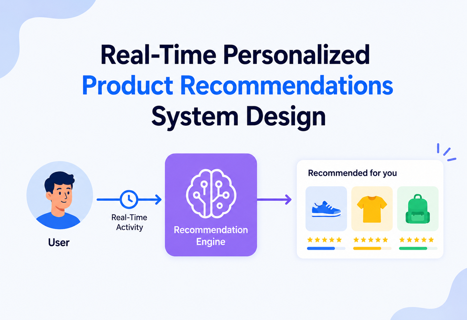
Real-Time Personalized Product Recommendations
How to architect the “Recommended for you” rail on an e-commerce homepage — a system that must blend a shopper’s lifetime purchase history with what they clicked thirty seconds ago, rank thousands of candidate products in under 100 milliseconds, and do this for tens of millions of shoppers simultaneously.
Introduction & History
Open any major shopping app and the homepage rarely shows the same products to two different people. One shopper sees running shoes and protein powder; another sees baby products and board books. That row of tiles — usually labeled “Recommended for you,” “Because you viewed…,” or “Customers also bought” — is the visible tip of a large, mostly invisible engine: a recommendation system.
A recommendation system is software that predicts which items a specific person is most likely to want, out of a catalog that may contain millions of options, and does so fast enough to render before the page finishes loading. A real-time recommendation system goes one step further: it factors in what the shopper is doing right now — the product they just clicked, the search they just typed — not just their history from last month.
Real-life analogy: imagine walking into a physical store where an attentive salesperson has memorized everything you’ve ever bought there, glances at what’s currently in your hand, and instantly points you toward three more things you’d probably like — before you’ve even asked. Now imagine that salesperson serving fifty million customers at the exact same moment, each getting a different, instantly-updated set of suggestions. That’s the engineering problem this tutorial solves.
A short history
Tapestry — the first “collaborative filtering” system
Xerox PARC researchers built Tapestry to filter email using other people’s ratings of messages, coining the term “collaborative filtering” — the foundational idea that people with similar past behavior will like similar future things.
GroupLens — academic collaborative filtering for Usenet
GroupLens formalized user-based collaborative filtering algorithms that are still taught in every recommender-systems course today.
Amazon’s item-to-item CF
Amazon published its item-to-item collaborative filtering approach, which scaled far better than user-based approaches because the relationships between items change much more slowly than the relationships between users.
Netflix Prize — matrix factorization goes mainstream
Netflix’s $1M open competition to improve its recommendation accuracy popularized matrix factorization techniques (like SVD) as a superior way to model latent user and item preferences.
Deep learning & embeddings — neural recommenders
Large platforms shifted to deep neural networks that learn dense vector “embeddings” for users and items, enabling similarity search across millions of products using nearest-neighbor techniques instead of hand-crafted rules.
Real-time, session-based recommendations — from “last month” to “last click”
Streaming infrastructure (Kafka, Flink) made it practical to fold a shopper’s actions from the last few seconds directly into their recommendations, not just their historical profile — the shift this tutorial focuses on.
A tiny online store with 200 products and 500 customers can get away with a simple rule: “show the 10 best-selling products to everyone.” But once that store has 10 million products and 50 million shoppers, “best-selling overall” stops being useful — the goal shifts to “best-selling for this specific person, right now,” and that shift is what turns a simple SQL query into a full-blown distributed machine learning system.
Problem & Motivation
Recommending products sounds simple in one sentence — “show people things they’ll like” — but building it at e-commerce scale means solving several genuinely hard problems simultaneously.

Candidate explosion
A catalog of 10 million products cannot be scored one-by-one for every homepage load — that would take far too long. We need a fast way to narrow millions of products down to a few hundred plausible candidates before doing any expensive ranking.
Real-time signal ingestion
A shopper who just viewed hiking boots should see that reflected in their recommendations within seconds, not after an overnight batch job. This demands a streaming pipeline, not just periodic database updates.
The cold-start problem
Brand-new shoppers have no history, and brand-new products have no purchase data. The system needs fallback strategies (popularity-based, content-based) for both, or it recommends nothing useful to a huge slice of traffic.
Latency budget
The entire pipeline — fetch candidates, score them, rank them, return them — must complete in well under 100 ms so it doesn’t delay homepage rendering, even though the underlying models can be computationally expensive.
Freshness vs. stability
Recommendations that change too wildly (a different set every reload) feel erratic and untrustworthy; recommendations that never change feel stale and ignore real-time intent. Balancing these is a genuine product and modeling challenge.
Feedback loops & bias
If the model only ever recommends what’s already popular, popular items get more clicks, which reinforces the model into recommending them even more — starving new or niche products of any visibility. This must be actively corrected for, not ignored.
The hard part of recommendations isn’t the machine learning model — it’s building a pipeline that can go from “user just clicked this” to “here are their next 20 personalized recommendations” in under a second, at a scale of hundreds of thousands of events per second.
- “Walk me through what happens end-to-end from the moment a user clicks a product to their homepage recommendations updating.”
- “How would you design recommendations differently for a brand-new user with zero history?”
- “Where would you accept staleness in this system, and where would you never accept it?”
Core Concepts
3.1 Two-stage recommendation: candidate generation + ranking
What: almost every production recommendation system splits the problem into two stages. Candidate generation quickly narrows millions of products down to a few hundred plausible ones using cheap, approximate methods. Ranking then takes those few hundred candidates and scores each one precisely with a more expensive model, keeping only the top 10–20 to actually display.
Analogy: think of hiring for a job. You don’t run a rigorous, multi-hour interview on every one of 10,000 applicants — you first do a cheap resume screen to get down to 50 candidates (candidate generation), then run detailed interviews only on those 50 (ranking). Running the expensive process on everyone would be far too slow and expensive; skipping the cheap filter and interviewing randomly would miss great candidates.
Practical example: candidate generation might use approximate nearest-neighbor search over item embeddings to find “500 products similar to what this user has browsed,” while ranking runs a gradient-boosted or neural click-through-rate model on just those 500 to pick the final 12 shown on the homepage.
3.2 Embeddings & vector similarity
What: an embedding is a list of numbers (a vector) that represents a user or a product in a way that captures meaning — products that are conceptually similar (two brands of running shoes) end up as vectors that are mathematically close together, even if they share no text in common.
Why it matters: once users and products live in the same vector space, “find products this user might like” becomes a nearest-neighbor search problem — extremely fast to compute at scale using specialized indexes (covered in Chapter 13), instead of comparing raw purchase histories directly.
Software example: a product embedding might be learned from a neural network trained on co-purchase and co-view data, such that “hiking boots” and “trail running shoes” end up near each other in the vector space, while “hiking boots” and “kitchen blender” end up far apart.
3.3 Collaborative filtering vs. content-based filtering
Collaborative filtering recommends based on patterns across many users: “people who bought what you bought also bought this.” It needs no understanding of the product itself — only behavioral data — but struggles with brand-new products that have no interaction history yet (cold start).
Content-based filtering recommends based on the attributes of items themselves: category, brand, price range, text description. It handles new products gracefully (a new product still has attributes) but tends to over-narrow recommendations to “more of exactly the same thing.”
Production systems almost always blend both approaches, using content-based signals to bootstrap cold-start cases and collaborative signals to capture patterns content alone can’t see.
3.4 Session-based / real-time personalization
What: rather than relying only on a user’s long-term profile (built from months of history), session-based recommendation weighs recent, in-session behavior heavily — what they’ve clicked, searched, or added to cart in just the last few minutes.
Analogy: imagine two customers with identical purchase histories from the past year. One is currently browsing camping gear; the other is browsing office furniture. A good system should show them very different homepages right now, even though their long-term profiles look the same — that’s what session-based personalization captures and long-term-only models miss.
3.5 Feature store
What: a feature store is a centralized system that computes, stores, and serves the input features (numbers describing a user, product, or context) used by machine learning models, ensuring the exact same feature values and computation logic are used both when training a model offline and when serving predictions online in real time.
Why it matters: without a feature store, teams often compute features slightly differently in training pipelines versus production serving code — a bug class called training-serving skew that silently degrades model accuracy in ways that are very hard to detect. The feature store exists specifically to eliminate this class of bug.
3.6 A/B testing & multi-armed bandits
What: because “is this a better recommendation model” is ultimately a business question (does it increase clicks, conversions, revenue), new ranking models are rarely shipped to 100% of traffic immediately. A/B testing splits traffic between the old and new model and compares business metrics statistically. Multi-armed bandit algorithms go further, dynamically shifting more traffic toward whichever model variant is currently performing best, balancing exploration (trying new variants) against exploitation (using the known-best variant).
3.7 CAP theorem applied to this system
What: the CAP theorem says that during a network partition, a distributed system must choose between Consistency (every reader sees the same, latest data) and Availability (every request gets a response, even if slightly stale). You cannot have perfect versions of both at once during a partition.
Where we choose Availability (AP): the online Feature Store and recommendation cache. If a replica is briefly unreachable, showing a shopper recommendations based on features that are a few seconds stale is far better than showing an error or a blank homepage — availability wins decisively here.
Where we lean toward Consistency (CP): inventory and pricing data feeding into candidate filtering. Recommending an item that’s actually out of stock or displaying an outdated price directly damages trust and can create real customer-service problems, so this path favors freshness and correctness over raw availability, even at a small latency cost.
Analogy: think of a store’s “sale ends today” sign. It’s fine if a shopper’s personalized suggestions are drawn from slightly stale browsing data, but it’s not fine if the price tag itself is wrong — one is a soft signal that can tolerate lag, the other is a hard fact the shopper will act on directly.
3.8 Concurrency & atomic counters
What: click and impression counters that feed into features like “click-through rate over the last hour” are updated by potentially tens of thousands of concurrent events per second for a popular product. A naive read-modify-write update loses updates under concurrency — the classic lost update problem.
Solution: counters use atomic increment operations (Redis’s INCR, or a stream aggregation framework’s built-in windowed counting) rather than application-level read-modify-write, guaranteeing correctness under high concurrency without explicit locking. For extremely hot products, increments are batched in memory for a short window and flushed periodically, trading a small amount of real-time precision for a large reduction in write load on the underlying store.
3.9 Consensus in the underlying infrastructure
What: several components this system depends on — the Kafka cluster’s controller broker, a Redis Cluster’s failover coordination — rely on consensus algorithms (typically Raft) to agree on a single leader node and avoid a split-brain scenario where two nodes both believe they’re authoritative after a network partition.
Why it matters here: application engineers building the recommendation pipeline don’t implement Raft themselves — they choose managed or battle-tested infrastructure that already solves this correctly. Recognizing when to build custom logic versus rely on proven consensus implementations is itself an important system design skill.
- “Why split into candidate generation and ranking instead of scoring the entire catalog directly?”
- “How would you handle a brand-new product with zero purchase history?”
- “What is training-serving skew, and how does a feature store prevent it?”
- “Where in this system would you favor CP over AP, and why does that specific data deserve stronger consistency?”
- “How would you prevent a lost update on a product’s real-time click counter under high concurrency?”
Architecture & Components
Below is the end-to-end architecture for the real-time recommendation system. Every box names the actual infrastructure component it represents, so it’s always clear what piece of the system is doing what.
4.1 Component-by-component breakdown
Load Balancer (L4/L7)
What it does: distributes incoming homepage requests across a fleet of API Gateway instances using an algorithm such as least-connections or weighted-latency, terminates TLS so backend services don’t each manage certificates, and continuously health-checks instances, pulling unhealthy ones out of rotation automatically.
Analogy: the load balancer is the maître d’ at a restaurant, glancing at which tables (server instances) have capacity and seating the next guest (request) at whichever one can serve them fastest.
Production example: AWS Application Load Balancer or an Envoy/NGINX fleet spread across multiple availability zones, so a single data-center failure never takes recommendations offline entirely.
API Gateway
What it does: the single front door for every client request — authenticates the caller, enforces per-user rate limits, routes to the correct downstream service by URL path, and validates request shape before business logic ever runs. It’s also where API versioning lives, so mobile apps on older versions keep working while new capabilities roll out.
Production example: Kong or AWS API Gateway, frequently paired with a service mesh (Istio/Linkerd) for encrypted, observable internal traffic.
Recommendation API Service
What it does: the orchestrator. It first checks the Cache Layer for a recently precomputed set of recommendations; on a miss, it calls the Experimentation Service to determine which model variant this user should see, then coordinates the candidate generation and ranking stages, and finally assembles and returns the response — all within the system’s overall latency budget.
Candidate Generation Service
What it does: quickly narrows the full catalog down to a few hundred plausible products using approximate nearest-neighbor search against the Vector Database (find products similar to the user’s embedding), plus rule-based candidate sources (trending items, same-category browsing history, inventory-in-stock filters).
Ranking Service
What it does: takes the candidate list and scores each product precisely using a more expensive model — predicting click-through and conversion probability — by pulling real-time features from the Feature Store and calling the Model Serving Layer for inference, then returns a ranked top-N list.
Feature Store (online + offline)
What it does: the online store serves low-latency feature lookups (a user’s recent click count, a product’s current stock level) during live ranking; the offline store holds the same features historically for training future model versions — guaranteeing training and serving use identical feature definitions.
Vector Database (ANN index)
What it does: stores dense embedding vectors for users and products and supports extremely fast approximate nearest-neighbor search — “find the 500 products whose embeddings are closest to this user’s embedding” — across millions of items in single-digit milliseconds.
Event Streaming Platform (Kafka)
What it does: ingests every click, product view, add-to-cart, and purchase event from clients in real time, acting as the durable backbone that decouples event producers (the client-facing services) from event consumers (the stream processor, analytics, and training pipelines).
Stream Processor (Flink)
What it does: consumes the raw event stream and computes real-time aggregated features (session click count, time since last purchase, category affinity in the last 10 minutes), writing them continuously into the online Feature Store so ranking always sees up-to-the-second signals.
Model Serving Layer
What it does: hosts trained ranking and embedding models behind a low-latency inference API, optimized (via batching, GPU acceleration, or quantization) to return predictions within the tight per-request latency budget the Ranking Service depends on.
Offline Training Pipeline
What it does: periodically (e.g., daily) retrains ranking and embedding models on historical interaction data pulled from the Interaction DB and offline Feature Store, then publishes new model versions to the Model Registry.
Model Registry
What it does: tracks every trained model version with its metadata (training data snapshot, evaluation metrics, deployment status), giving the Model Serving Layer a controlled, auditable source for which model version is currently live.
Experimentation Service
What it does: assigns each user to an A/B test bucket or bandit arm, ensuring consistent assignment across requests (the same user always sees the same model variant during an experiment) and feeding outcome data back for statistical analysis.
Cache Layer (Redis Cluster)
What it does: stores precomputed recommendation lists for a short TTL and hot feature lookups, absorbing the majority of homepage load requests before they ever reach the candidate generation and ranking stages.
Catalog DB & Interaction DB
What it does: the Catalog DB (sharded relational store) holds structured product metadata, pricing, and inventory; the Interaction DB (wide-column store) holds the massive volume of raw click/view/purchase events at the throughput a relational database can’t sustain.
Monitoring Stack
What it does: every service emits metrics, structured logs, and distributed traces into a centralized observability stack, giving engineers a single place to diagnose latency spikes or model quality regressions.
- “Why separate Candidate Generation from Ranking into two services instead of one?”
- “What happens to the homepage if the Model Serving Layer is briefly unavailable?”
- “Why maintain both an online and an offline Feature Store instead of just one?”
- “How does the API Gateway protect the Ranking Service from a sudden traffic spike, e.g. during a flash sale?”
Internal Working
5.1 Serving a homepage recommendation request
Notice the short 30-second cache TTL on the assembled recommendation list. This is a deliberate balance: it’s long enough to absorb repeated homepage reloads and back-button navigation cheaply, but short enough that a user’s very next click (processed asynchronously through the streaming pipeline) can influence what they see again within roughly half a minute — an acceptable trade-off between raw freshness and system load.
5.2 Real-time feature computation
The Stream Processor (Flink) maintains a small, continuously updated window of each active user’s recent behavior — typically the last 10–30 minutes of a session — and writes aggregated features into the online Feature Store the moment new events arrive, rather than waiting for a batch job.
public class SessionFeatureAggregator extends KeyedProcessFunction<String, ClickEvent, FeatureUpdate> {

    private ValueState<SessionAggregate> sessionState;

    @Override
    public void processElement(ClickEvent event, Context ctx, Collector<FeatureUpdate> out) {
        SessionAggregate agg = sessionState.value();
        if (agg == null) {
            agg = new SessionAggregate(event.getUserId());
        }

        agg.recordClick(event.getProductId(), event.getCategory(), event.getTimestamp());
        agg.expireOlderThan(event.getTimestamp() - Duration.ofMinutes(15).toMillis());

        sessionState.update(agg);

        // Emit an incremental feature update - consumed by the online Feature Store writer
        out.collect(new FeatureUpdate(
            event.getUserId(),
            agg.getTopCategoryLast15Min(),
            agg.getClickCountLast15Min(),
            agg.getLastViewedProductId()
        ));
    }
}
Explanation: keyed state (per user_id) lets Flink maintain a live, continuously-expiring rolling window without needing to re-scan historical events on every update. The output — top_category_last_15_min, click_count_last_15_min, last_viewed_product_id — is exactly the kind of real-time feature that separates session-based personalization from a system relying only on last night’s batch-computed profile.
- “Why cache the final recommendation list for only 30 seconds instead of, say, 30 minutes?”
- “How does keyed state in Flink avoid re-scanning a user’s full event history on every click?”
5.3 Assembling features for ranking
Before calling the Model Serving Layer, the Ranking Service must assemble a feature vector for every candidate product, combining real-time session features, static product attributes, and user-product affinity signals into the exact shape the model expects.
public class FeatureAssembler {

    public List<FeatureVector> assemble(String userId, List<String> candidateIds) {
        UserFeatures userFeatures = featureStore.getUserFeatures(userId);
        Map<String, ProductFeatures> productFeatures =
            featureStore.getProductFeaturesBatch(candidateIds); // one batched call, not N calls

        List<FeatureVector> vectors = new ArrayList<>();
        for (String productId : candidateIds) {
            ProductFeatures pf = productFeatures.get(productId);
            double affinity = affinityStore.getUserProductAffinity(userId, pf.getCategory());

            vectors.add(FeatureVector.builder()
                .productId(productId)
                .sessionClickCount(userFeatures.getSessionClickCountLast15Min())
                .topSessionCategory(userFeatures.getTopCategoryLast15Min())
                .productPrice(pf.getPrice())
                .productPopularityScore(pf.getPopularityScore())
                .inStock(pf.isInStock())
                .categoryAffinity(affinity)
                .build());
        }
        return vectors;
    }
}
Explanation: the batched product-feature lookup (getProductFeaturesBatch) is deliberate — issuing one network call per candidate instead of one batched call for all 500 candidates would blow through the latency budget through sheer round-trip overhead alone. This same “batch, don’t loop” principle applies to the subsequent Model Serving call as well.
Data Flow & Lifecycle
6.1 The full event lifecycle
Event emission
Client emits a click/view/add-to-cart/purchase event; it’s sent asynchronously so it never blocks the user’s page interaction.
Ingestion
Event lands on a Kafka topic partitioned by user_id, preserving per-user event ordering.
Real-time feature update
Flink consumes the event, updates the user’s session aggregate, and writes fresh features to the online Feature Store — typically within 1–2 seconds.
Durable storage
The raw event is also persisted to the Interaction DB (wide-column store) for later use in offline model training and analytics.
Next recommendation request
The next time this user’s homepage requests recommendations (cache miss after the 30s TTL expires), the Ranking Service pulls the freshly updated real-time features and reflects the new behavior in the ranked output.
Nightly batch retraining
The Offline Training Pipeline aggregates the day’s accumulated interaction data, retrains embedding and ranking models, evaluates them against held-out data, and — if they beat the current production model on offline metrics — registers them in the Model Registry as candidates for a canary rollout.
Embedding refresh
Updated product and user embeddings are recomputed and reloaded into the Vector Database, so candidate generation reflects the latest learned relationships between products.
6.2 Batch vs. streaming: where each is used
| Task | Batch or streaming? | Why |
|---|---|---|
| Session-level features (recent clicks, current category interest) | Streaming | Must reflect behavior from seconds ago to power session-based personalization |
| Model training (ranking & embedding models) | Batch | Needs large, stable historical datasets; retraining every few seconds would be wasteful and unstable |
| Long-term user profile features (lifetime purchase categories) | Batch (daily) | Changes slowly; daily freshness is more than sufficient |
| Inventory / price updates | Streaming (near-real-time) | Recommending an out-of-stock or mispriced product directly damages user trust |
A frequent mistake is letting the online Feature Store and offline training pipeline compute the “same” feature using subtly different code paths — for example, a 15-minute rolling window in production versus a calendar-hour bucket in training. This training-serving skew silently degrades model quality without throwing any errors, which is exactly why a shared feature store with one definition per feature is treated as a core architectural requirement, not a nice-to-have.
6.3 The two-stage funnel, visualized
Advantages, Disadvantages & Trade-offs
✓ Advantages of this architecture
- Two-stage candidate generation + ranking keeps latency bounded regardless of catalog size
- Streaming feature pipeline enables genuinely real-time personalization, not just daily-batch profiles
- Feature store eliminates training-serving skew by sharing one feature definition across training and serving
- Model registry + canary rollout lets new models ship safely without risking the whole homepage
- Cache-first serving absorbs the vast majority of homepage load without touching the ML pipeline at all
× Disadvantages & costs
- Significant infrastructure and operational complexity — streaming, feature stores, vector databases, and model serving all need dedicated expertise
- Real-time feature pipelines are harder to debug than simple batch jobs when something goes subtly wrong
- Higher infrastructure cost than a simple “popular items” fallback, especially at low scale
- Model quality requires ongoing investment (retraining, monitoring, experimentation) — it’s never “done”
- Feedback-loop bias must be actively monitored and corrected, or the system quietly narrows what it ever recommends
7.1 Key trade-off decisions
| Decision | Option A | Option B | What we chose & why |
|---|---|---|---|
| Candidate generation | Score entire catalog | ANN search over embeddings | ANN search — scoring 10M+ products directly per request is far too slow for a <100 ms budget |
| Feature freshness | Daily batch only | Real-time streaming | Streaming for session signals, batch for stable long-term profile — a hybrid that balances cost and freshness |
| Recommendation cache TTL | No caching (always fresh) | Long TTL (minutes+) | Short TTL (~30s) — balances system load against acceptable staleness |
| Model rollout | Full cutover to new model | Canary + A/B test | Canary/A-B — a regression in a ranking model directly costs revenue, so blast radius must be limited |
| Cold-start handling | Show nothing until enough data exists | Fallback to popularity/content-based | Fallback — an empty or generic homepage for new users is worse than an imperfect but reasonable one |
- “What would break if you removed the candidate generation stage and tried to rank the whole catalog directly?”
- “Justify the 30-second cache TTL — what happens if it’s too long, and what happens if it’s too short?”
Performance & Scalability
8.1 The latency budget
Every component in the synchronous serving path shares one strict overall budget — typically under 100 ms end-to-end. Breaking this down helps clarify why each stage exists and what it’s allowed to cost:
| Stage | Target latency | Why it’s feasible |
|---|---|---|
| API Gateway auth + routing | ~2–5 ms | Token validation is cheap and stateless |
| Cache lookup (hit path) | ~1–3 ms | In-memory Redis read |
| ANN candidate search | ~10–20 ms | Approximate nearest-neighbor indexes trade a small accuracy loss for massive speed gains over exact search |
| Feature store lookup | ~5–10 ms | Online store is optimized purely for low-latency key-based reads |
| Model inference (ranking) | ~20–40 ms | Batched GPU/optimized inference on only a few hundred candidates, not the whole catalog |
| Assembly & response | ~5 ms | Simple in-memory sort and serialization |
8.2 Horizontal scaling of stateless services
The API Gateway, Recommendation API, Candidate Generation Service, and Ranking Service are all stateless — no instance holds data another instance lacks access to. Scaling under load means adding more instances behind the Load Balancer, coordinated by an auto-scaler watching CPU, request latency, or queue depth for the streaming side.
8.3 Why approximate nearest-neighbor, not exact search
What: finding the mathematically closest vectors to a query vector exactly requires comparing against every single item — O(n) per query, which is far too slow across millions of products. Approximate nearest-neighbor (ANN) algorithms (like HNSW graphs or product quantization) build an index structure that finds vectors that are almost certainly among the closest matches, in roughly logarithmic time, trading a small, usually imperceptible accuracy loss for orders-of-magnitude speed gains.
Analogy: exact search is like reading every book in a library to find the ten most similar to the one you’re holding. ANN search is like using the library’s subject catalog to jump straight to the right section first — you might occasionally miss one perfect match shelved oddly, but you find excellent matches almost instantly instead of after hours of reading.
8.4 Applying Little’s Law to capacity planning
Little’s Law (L = λ × W) tells us the number of concurrent in-flight requests (L) equals arrival rate (λ) times average processing time (W). If the platform expects 200,000 recommendation requests/sec at peak and each takes 80 ms end-to-end, the system needs capacity for roughly 16,000 concurrent in-flight requests at any instant — a number that directly drives how many Ranking Service instances, model-serving replicas, and connection-pool slots must be provisioned ahead of a known peak event like a flash sale.
8.5 Auto-scaling triggers in practice
Rather than scaling purely on CPU utilization (a lagging indicator for this workload), the Ranking Service and Candidate Generation Service scale on a blend of signals: request queue depth (a leading indicator that latency is about to degrade), p95 latency trending upward, and scheduled pre-scaling ahead of known traffic events like flash sales or major shopping holidays, where historical traffic patterns are used to warm up extra capacity before the event starts rather than reacting only after load has already arrived.
The Model Serving Layer, when running on GPU-backed infrastructure, scales more conservatively than the CPU-bound services, since GPU node provisioning takes longer — this asymmetry is why maintaining a modest baseline of “warm” GPU capacity above the immediate minimum is often more cost-effective than aggressively scaling GPU nodes to zero during quiet periods.

- “Walk me through the latency budget for a single recommendation request and where you’d look first if p99 latency doubled.”
- “Why is ANN search an acceptable trade-off here, when it can occasionally miss the mathematically closest item?”
- “Why might you pre-scale ahead of a known traffic event rather than relying purely on reactive auto-scaling?”
High Availability & Reliability
9.1 Redundancy at every layer
- Multi-AZ deployment: every stateless service and the Load Balancer run across at least three availability zones.
- Feature store replication: the online feature store (typically Redis- or key-value-backed) runs with replica nodes per shard for automatic failover.
- Kafka replication: event topics use a replication factor of 3, so a single broker failure doesn’t lose in-flight click/purchase events.
- Model serving redundancy: multiple replicas of each active model version run behind the Model Serving Layer’s own internal load balancing, so one replica crashing never causes a visible latency spike.
9.2 Graceful degradation
| What fails | Degraded behavior |
|---|---|
| Vector Database unavailable | Candidate Generation falls back to rule-based candidates (trending items, same-category browsing history) instead of failing the whole request |
| Model Serving Layer unavailable | Ranking Service falls back to a simpler, cached popularity-based ordering rather than returning an error |
| Feature Store (online) unavailable | Ranking proceeds using only static/content-based features, sacrificing personalization freshness but not availability |
| Stream Processor down | Real-time features stop updating, but stale features continue serving; events buffer safely in Kafka for reprocessing once recovered |
9.3 Circuit breakers & bulkheads
Every synchronous cross-service call (Ranking Service → Model Serving, Candidate Generation → Vector DB) is wrapped in a circuit breaker with a fallback path, and separate connection/thread pools per downstream dependency (the bulkhead pattern) ensure a slow Vector Database can never starve the resources needed to serve a fast cache-hit request.
A recommendation system failure should degrade recommendation quality, never break the homepage itself. Every stage in the pipeline has a defined fallback (cache → rule-based candidates → popularity ranking → empty-but-valid response), so the worst-case outcome under a cascading outage is a generic “trending now” rail — never a broken page.
9.4 Disaster recovery & multi-region considerations
Cross-region backups of the Catalog DB, Interaction DB, and Model Registry run continuously, with a documented Recovery Point Objective (RPO) under 5 minutes and Recovery Time Objective (RTO) under 30 minutes for a full regional failover. For a globally distributed platform, the Model Serving Layer and Feature Store are typically deployed per-region, with each region serving traffic from its nearest data center to keep the latency budget achievable — a request routed cross-continent to a distant region would blow through the sub-100 ms target on network transit time alone, regardless of how fast the pipeline itself runs.
Vector Database and trained model artifacts are replicated across regions asynchronously after each training/embedding-refresh cycle, since these change on a predictable batch schedule and don’t need synchronous cross-region consistency the way a live transaction would.
- “If the Model Serving Layer is completely down, what does the user actually see, and why is that acceptable?”
- “How does a circuit breaker around the Vector DB call prevent a slow dependency from taking down the whole homepage?”
Security
10.1 Authentication & authorization
Every homepage request carries a short-lived JWT validated at the API Gateway before reaching any downstream service. Recommendation results are always scoped to the authenticated user’s ID server-side — the client never supplies which user’s recommendations to fetch, preventing one user from requesting another user’s personalized data.
10.2 Protecting user behavioral data
Click, view, and purchase events are among the most sensitive data an e-commerce platform holds, since they can reveal health conditions, financial situation, or other personal circumstances through purchase patterns. This drives several requirements:
- Encryption in transit: TLS 1.2+ everywhere, including internal service-to-service traffic via mutual TLS (mTLS) within the service mesh.
- Encryption at rest: the Interaction DB and Feature Store volumes are encrypted with AES-256, keys managed by a dedicated key management service.
- Data minimization: the Feature Store retains only aggregated behavioral signals needed for ranking, not indefinitely-retained raw event logs, reducing exposure if a breach occurs.
- Access control: only the Ranking Service and offline training jobs can read raw interaction data — no engineer or ad-hoc dashboard queries directly against production behavioral data without going through an audited access process.
10.3 Compliance & the right to be forgotten
GDPR/CCPA-style deletion requests must cascade across every store that touches a user’s data — the Interaction DB, both Feature Stores, cached recommendation lists, and any embeddings derived from that user’s behavior. A “delete my data” request triggers an async job that purges or anonymizes records across all of these, and any model that was trained on that user’s raw data must be handled per the platform’s data-retention policy (typically, models are retrained periodically anyway, which naturally ages out deleted users’ influence, but explicit purging of cached/served data must happen immediately, not just on the next retrain).
10.4 Rate limiting & abuse protection
The API Gateway enforces per-user and per-IP rate limits using a token-bucket algorithm to prevent scraping attacks (a competitor or bot systematically querying recommendations to reverse-engineer the catalog or pricing strategy) without disrupting normal user browsing patterns.
10.5 Adversarial manipulation
| Threat | Mitigation |
|---|---|
| Click fraud to artificially boost a product’s ranking | Anomaly detection on click patterns (velocity, device fingerprint diversity) before events are trusted as training signal |
| Scraping recommendations to reverse-engineer catalog/pricing | Rate limiting, bot detection, and response randomization within an acceptable quality range |
| Data poisoning via fake accounts generating fabricated interaction history | Account-age and behavioral-consistency checks before interaction data is weighted heavily in training |
- “How would you prevent a seller from gaming the recommendation ranking with fake clicks on their own products?”
- “Walk me through what has to happen across the system when a user requests full account and data deletion.”
Monitoring, Logging & Metrics
11.1 The three pillars of observability
Prometheus + Grafana
Tracks request rate, error rate, and p50/p95/p99 latency (the “RED” method) per service, plus business/ML metrics like click-through rate, conversion rate, and cache hit rate. Grafana dashboards visualize these in real time.
Structured JSON → ELK / OpenSearch
Structured JSON logs, tagged with a correlation ID, ship to an ELK/OpenSearch stack so a single request can be traced across every service it touched.
OpenTelemetry distributed tracing
Distributed tracing shows exactly how long each hop took — API Gateway → Recommendation API → Candidate Generation → Vector DB — making latency regressions easy to localize.
11.2 Model-quality monitoring — a category beyond standard system metrics
Unlike most backend systems, this one needs monitoring for a failure mode standard infrastructure metrics won’t catch: the model can be technically “healthy” (fast, no errors) while quietly recommending badly. This requires dedicated ML-quality monitoring:
- Prediction drift: comparing the distribution of the model’s live output scores against its training-time distribution, flagging when they diverge meaningfully.
- Feature drift: monitoring whether incoming feature values (e.g., average session click count) shift significantly from what the model was trained on — often an early warning sign before business metrics degrade.
- Online business metrics: click-through rate, add-to-cart rate, and conversion rate tracked continuously per model version, alerting if a newly rolled-out model underperforms the previous one.
Alerting only on infrastructure metrics (latency, error rate) and not on model-quality metrics means a genuinely broken recommendation model — one that’s fast, returns 200 OK every time, but is recommending irrelevant products — can run in production for days before anyone notices, usually only after a business stakeholder asks why conversion rates dropped.
11.3 Key alerts
- End-to-end p99 latency exceeding the recommendation SLA (e.g., >150 ms) for a sustained window
- Recommendation cache hit rate dropping below target (signals a cache eviction storm or a sudden traffic pattern shift)
- Kafka consumer lag on the event-ingestion topic growing unbounded (signals the Stream Processor can’t keep up)
- Online click-through rate for the current production model dropping significantly versus its rolling 7-day baseline
- Feature drift score crossing a configured threshold for any feature feeding the ranking model
- Vector Database query latency or error rate crossing a threshold (early warning before candidate generation starts timing out)
- “How would you detect that a newly deployed ranking model is technically healthy but recommending poorly?”
- “What’s the difference between feature drift and prediction drift, and why monitor both?”
Deployment & Cloud Strategy
12.1 Containerization & orchestration
Every microservice ships as a Docker container running on Kubernetes, which handles scheduling, auto-scaling (via Horizontal Pod Autoscaler watching CPU and custom metrics like request queue depth), self-healing, and rolling deployments. The Model Serving Layer often runs on GPU-backed node pools, scaled independently from the CPU-bound API services.
12.2 Deployment strategy: shadow deployments + canary releases
New ranking models go through an extra safety stage beyond standard software canaries: a shadow deployment, where the new model receives a copy of live production traffic and produces predictions that are logged and compared against the current model’s outputs — but never actually shown to users. Only once the shadow model’s offline-evaluated quality and latency look healthy does it proceed to a real canary (5% of live traffic, gradually increasing) with actual business-metric monitoring.
12.3 The CI/CD pipeline for models vs. services
| Artifact | Pipeline |
|---|---|
| Application code (API Gateway, Recommendation API, etc.) | Standard CI/CD: lint, test, build container, canary rollout on Kubernetes |
| ML models (ranking, embeddings) | Training pipeline: offline evaluation against held-out data → shadow deployment → canary → full rollout, gated by both engineering and data-science review |
12.4 Infrastructure as Code
Kubernetes clusters, Kafka topics, the Vector Database cluster, and Feature Store infrastructure are all defined declaratively via Terraform, version-controlled, and applied through a reviewed CI/CD pipeline for reproducibility across environments.
- “Why add a shadow deployment stage before a canary, instead of going straight to a canary?”
- “Why would the Model Serving Layer scale independently from the rest of the API services?”
Databases, Caching & Load Balancing in Depth
13.1 Why different stores for different data
| Data | Store | Reasoning |
|---|---|---|
| Product catalog metadata | Sharded PostgreSQL | Structured, relatively low write volume, benefits from relational integrity and transactional pricing/inventory updates |
| Raw interaction events (clicks, views, purchases) | Cassandra / DynamoDB (wide-column) | Extremely high write volume, append-heavy, simple partition-key access pattern |
| User & item embeddings | Vector Database (FAISS/HNSW/Milvus) | Purpose-built for approximate nearest-neighbor search across millions of high-dimensional vectors — something relational/wide-column stores cannot do efficiently |
| Online features (real-time) | Redis / low-latency KV store | Sub-10 ms reads required on the ranking hot path |
| Offline features (training) | Data lake (Parquet on S3, queried via Spark) | Optimized for large-scale batch reads over historical data, not point lookups |
13.2 Replication & partitioning depth
The Interaction DB (wide-column store) is partitioned by user_id with a time-bucketed clustering key, so “get this user’s recent events” is a single efficient partition scan rather than a scatter-gather query. It runs with a replication factor of 3 and typically uses a tunable consistency level — QUORUM for writes (a majority of replicas must acknowledge) and ONE for most analytical reads, favoring low latency since a training job reading slightly stale data is an acceptable trade-off.
The Vector Database is sharded by a hash of product ID across nodes, with each shard replicated for both durability and read-throughput scaling, since ANN queries are read-heavy and benefit from parallelizing search across replicas.

13.3 ANN index trade-offs
Different ANN index types trade off differently: HNSW (Hierarchical Navigable Small World graphs) offers excellent query speed and recall at the cost of higher memory usage and slower index-build time; product quantization-based indexes (like IVF-PQ) use far less memory by compressing vectors, at some cost to recall accuracy. The choice depends on catalog size and available memory — a 10-million-product catalog with tight latency requirements commonly uses HNSW for the primary index, sometimes combined with quantization for very large deployments to control memory cost.
13.4 Load balancing beyond the edge
Internally, Kafka partitions distribute event load across Flink task instances; the Model Serving Layer load-balances inference requests across GPU replicas using request-queue-aware routing (favoring the least-busy replica rather than simple round-robin, since inference times can vary); and the Feature Store’s Redis Cluster uses hash-slot-based routing so key lookups land deterministically on the correct node without a central coordinator on the hot path.
13.5 Caching patterns used
Cache-aside
Used for the final assembled recommendation list — the Recommendation API checks Redis first, and on a miss runs the full pipeline and populates the cache.
Read-through for product metadata
Product detail lookups (price, image, availability) needed to render each recommended item are cached with automatic refresh on expiry, since this data changes more slowly than personalization signals.
TTL-based invalidation
Rather than explicit invalidation, the recommendation cache simply relies on a short TTL — appropriate here because staleness is naturally bounded and acceptable, unlike the strict correctness needs of, say, a moderation ban in other systems.
- “Why is a vector database necessary here instead of just running similarity search in the application layer?”
- “What’s the trade-off between HNSW and quantization-based ANN indexes, and how would catalog size influence your choice?”
APIs & Microservice Boundaries
14.1 Representative REST API surface
GET    /v1/homepage/recommendations              # get personalized homepage recs
GET    /v1/products/{id}/similar                 # "customers also viewed" for a product page
POST   /v1/events                                # client-emitted click/view/cart events
GET    /v1/experiments/assignment                # current A/B/bandit variant for this user
POST   /v1/models/{id}/deploy                    # (internal) promote a model to canary/full rollout
GET    /v1/models/{id}/metrics                   # (internal) online model-quality metrics
14.2 Why events are fire-and-forget from the client
The POST /v1/events endpoint is intentionally designed to respond immediately (202 Accepted) without waiting for the event to be processed by the streaming pipeline — the client should never feel a delay from emitting a click event. This is a direct application of the same synchronous-vs-asynchronous split covered earlier: user-facing latency depends only on the fast acknowledgment, not on downstream feature computation.
14.3 Microservice communication patterns
| Interaction | Pattern | Why |
|---|---|---|
| Recommendation API → Candidate Generation → Ranking | Synchronous gRPC | Results are needed immediately to assemble the response within the latency budget |
| Ranking Service → Model Serving Layer | Synchronous gRPC (often batched) | Inference must return before ranking can complete, but batching multiple candidates per call amortizes overhead |
| Client → Event Ingestion | Asynchronous, fire-and-forget (Kafka-backed) | Must never add latency to the user’s browsing experience |
| Client → Recommendation API | Synchronous REST/HTTPS | Standard client-facing contract, cacheable and versioned |
gRPC vs REST internally: the tight latency budget across candidate generation and ranking makes gRPC’s binary protocol and strongly-typed protobuf contracts a better fit than JSON/REST for internal service-to-service calls, where every millisecond of serialization overhead counts against the overall budget.
14.4 Backend-for-Frontend (BFF) considerations
Mobile clients often need a slightly different response shape than web clients — smaller product image variants, fewer metadata fields, different pagination sizes for a smaller screen. Rather than bloating the Recommendation API with client-specific branching logic, many implementations add a thin Backend-for-Frontend layer (or a GraphQL gateway) between the API Gateway and Recommendation API, letting each client type request exactly the fields and shape it needs without over-fetching data it will discard, and without coupling the core recommendation logic to presentation concerns.
- “Why does the event ingestion endpoint return immediately without waiting for the event to be fully processed?”
- “Why batch multiple candidates into one inference call to the Model Serving Layer instead of one call per candidate?”
- “When would you introduce a BFF layer, and what problem does it solve that the core Recommendation API shouldn’t have to?”
Design Patterns & Anti-patterns
15.1 Patterns used
Two-stage retrieval (funnel pattern)
Candidate generation narrows the search space cheaply before an expensive ranking model runs on a much smaller set — the core architectural pattern of nearly every large-scale recommender system.
Circuit breaker
Wraps every synchronous cross-service call, providing a defined fallback rather than letting a failure cascade and take down the whole homepage.
CQRS
Event writes (clicks, purchases) flow through Kafka into the Interaction DB and Feature Store, while reads (recommendation serving) flow through an entirely separate, read-optimized path — the two paths use different data shapes and different infrastructure by design.
Bulkhead
Separate connection/thread pools per downstream dependency (Vector DB, Model Serving, Feature Store) so one degraded dependency can’t exhaust resources needed by the rest of the request path.
Shadow deployment
A model-specific pattern where a new model runs against live traffic without affecting real users, letting teams validate quality and latency safely before any real exposure.
Strangler fig (for model rollouts)
New model versions gradually take over traffic share from the old one via canary percentages, rather than an instant cutover — the same incremental-replacement idea used for migrating legacy systems, applied to ML models.
15.2 Anti-patterns to avoid
× Computing features differently in training vs. serving
Writing separate feature-computation code for the offline training pipeline and the online serving path (instead of sharing one feature store definition) is the single most common cause of silent model-quality regressions in production recommendation systems.
× Scoring the entire catalog on every request
Skipping candidate generation and running the expensive ranking model against millions of products directly makes the latency budget impossible to hit — the two-stage funnel exists precisely to avoid this.
× Shipping a new model straight to 100% of traffic
Without shadow deployment and canary rollout, a regression in a new ranking model directly and immediately damages conversion rate for the entire user base before anyone notices.
- “Explain how CQRS applies to this system even though there’s no obvious ‘command’ in the traditional sense.”
- “Why is training-serving skew specifically dangerous compared to a normal software bug?”
Best Practices & Common Mistakes
16.1 Best practices
- Build the feature store and shared feature definitions in from day one — retrofitting one after training and serving have diverged is a painful, error-prone migration.
- Always have a defined, tested fallback for every stage of the pipeline (candidate generation, ranking, feature lookup) so infrastructure failures degrade quality rather than availability.
- Monitor model-quality metrics (drift, online CTR/CVR) with the same seriousness as infrastructure metrics — a “healthy” system can still be recommending poorly.
- Use shadow deployments before canaries for any model change, since offline evaluation metrics don’t always predict real-world business impact.
- Actively correct for feedback-loop bias (e.g., reserving a small percentage of recommendation slots for exploration) rather than letting the model only ever reinforce what’s already popular.
16.2 Common mistakes
Teams often optimize heavily for engaged, high-history users and treat new users and new products as an afterthought — but cold-start traffic is frequently a large fraction of daily visitors, and a poor cold-start experience directly costs first-purchase conversion.
A model that scores better on offline metrics (like AUC on held-out historical data) doesn’t always translate into better real-world business metrics, because historical data reflects what the previous model chose to show — this is why shadow deployment and live A/B testing remain essential, not optional, steps.
If inventory and pricing data isn’t kept sufficiently fresh in the serving path, the system can confidently recommend a product that’s actually sold out or displayed at a stale price — a fast, well-personalized, but factually wrong recommendation is often worse than a generic but accurate one.
Reserving recommendation slots for exploration has a real, measurable short-term cost — exploratory items generally convert worse than the model’s top-confidence picks. Engineering teams sometimes quietly remove exploration slots under pressure to improve short-term conversion metrics, which feels like a win in the current quarter but starves the model of the very data it needs to keep improving and correcting bias, ultimately hurting long-term recommendation quality.
- “How would you measure whether your cold-start fallback strategy is actually working well?”
- “Why might a model that wins on offline evaluation metrics still lose in a live A/B test?”
Real-World Industry Examples
Amazon
Popularized item-to-item collaborative filtering and continues to use a blend of collaborative and content-based signals across “customers also bought,” “frequently bought together,” and personalized homepage rails, each powered by somewhat different candidate generation strategies tuned to that specific placement.
Netflix
While a streaming platform rather than e-commerce, Netflix’s publicly documented architecture — separating candidate generation from ranking, and running extensive A/B testing infrastructure — is one of the most cited real-world blueprints for the two-stage pattern described in this tutorial.
Alibaba
Has published extensively on real-time, session-based recommendation at massive scale, including techniques for handling the extreme candidate-explosion problem across catalogs with hundreds of millions of products.
Etsy
Has documented its shift from purely batch-computed recommendations to real-time, session-aware personalization, citing measurable lifts in engagement directly attributable to incorporating last-few-minutes browsing signal — a concrete real-world validation of the session-based approach covered in Chapter 3.
Instacart
Combines real-time context (time of day, current cart contents) with historical purchase patterns for grocery reorder recommendations, an example of context-aware ranking beyond pure user/item similarity.
Spotify
Another non-e-commerce example whose “Discover Weekly” and real-time session-based “Radio” features are widely referenced for balancing exploration (new, unfamiliar recommendations) against exploitation (safe, known-good recommendations) — directly relevant to the feedback-loop bias problem discussed in Chapter 2.
Walmart
Has publicly discussed rebuilding its recommendation infrastructure around real-time streaming and a shared feature-store approach to reduce training-serving skew across dozens of independently-owned recommendation surfaces (homepage, search, cart page), a real-world illustration of why a single, shared Feature Store service matters once a platform has many different recommendation placements rather than just one.
A recurring theme across all of these companies’ public engineering writing is that the underlying architectural pattern — candidate generation, ranking, feature store, streaming pipeline, careful rollout — repeats across very different products (video, music, groceries, general retail), even though the specific models and business metrics differ substantially. This is a strong signal that the architecture in this tutorial reflects genuinely proven, reusable engineering practice rather than a one-off design choice specific to any single company.
- “What can an e-commerce recommendation system learn architecturally from a streaming platform like Netflix, despite the different domain?”
- “Why might grocery/reorder recommendations rely more heavily on context (time of day, current cart) than a general catalog browse recommendation would?”
Frequently Asked Questions
Why not just recompute recommendations from scratch on every single homepage load?
Running the full candidate generation and ranking pipeline for every single request would work, but a short cache layer absorbs the huge share of repeat homepage loads (back button, page refresh, opening a new tab) far more cheaply, freeing the ranking infrastructure’s capacity for requests that genuinely need fresh computation.
How do you personalize recommendations for a user who isn’t logged in?
Anonymous sessions are tracked via a temporary session/device identifier, and the same real-time streaming pipeline builds session-based features for that identifier — so personalization still works within a browsing session, it just resets rather than persisting long-term once the session ends (unless the user later logs in and the session is linked to their account).
What happens if the streaming pipeline falls behind during a huge traffic spike, like a flash sale?
Events buffer safely in Kafka rather than being dropped, since Kafka is designed to absorb bursts far above steady-state consumer throughput. The Feature Store simply serves slightly staler real-time features until the Stream Processor catches up, which the system tolerates gracefully by design rather than treating as an outage.
How do you avoid recommendations becoming an endless loop of “more of the same”?
By deliberately reserving a small percentage of recommendation slots for exploration — showing occasional items outside the user’s obvious pattern, chosen via the bandit-style exploration strategy described in Chapter 3 — which both improves long-term personalization quality and actively counters the feedback-loop bias problem from Chapter 2.
Is A/B testing enough, or do you need shadow deployments too?
A/B testing alone still exposes real users to a potentially broken model, even at just 5% of traffic. Shadow deployment catches obvious problems (crashes, wildly wrong scores, latency issues) with zero user exposure first, making the subsequent canary meaningfully safer — the two techniques are complementary, not redundant.
How often should the ranking model actually be retrained?
There’s no universal answer — it depends on how quickly catalog and user behavior shift. Fast-moving fashion or trend-driven catalogs often retrain daily; more stable catalogs (durable goods, appliances) may retrain weekly. The right cadence is usually determined empirically by monitoring how quickly offline evaluation metrics degrade between retraining cycles.
Why does the system need both a Vector Database and a traditional relational Catalog DB?
They answer fundamentally different questions. The Vector Database answers “which products are conceptually similar to this one” via embedding similarity — something a relational database cannot do efficiently. The Catalog DB answers “what is this product’s current price, description, and stock level” — structured facts that benefit from transactional guarantees the Vector Database doesn’t provide.
What’s the difference between the recommendation cache and the feature store, since both use Redis?
They store fundamentally different things at different layers. The recommendation cache stores the final, fully-computed output — a ranked list of product IDs ready to display. The online feature store stores the raw inputs (session click counts, category affinity scores) that the Ranking Service needs to compute that output in the first place. A cache miss on the recommendation cache still needs the feature store; a feature store update doesn’t automatically refresh the recommendation cache until its TTL expires.
Summary & Key Takeaways
Designing a real-time recommendation system is fundamentally an exercise in balancing three tensions: a tight latency budget vs. the computational cost of accurate ranking, real-time freshness vs. system stability, and personalization quality vs. exploration/fairness across the catalog. The architecture in this tutorial resolves those tensions through a two-stage candidate-generation-plus-ranking funnel, a shared feature store that eliminates training-serving skew, a streaming pipeline that folds in-session behavior into ranking within seconds, and a disciplined shadow-then-canary rollout process that keeps model changes safe.
It’s worth restating why each major design decision exists, because interview settings often probe exactly this: sharding and caching exist because catalog and traffic scale demand it; the streaming pipeline exists because a shopper’s intent changes faster than any daily batch job could capture; the feature store exists because training and serving must agree on what a “feature” means; and the shadow-canary rollout discipline exists because a bad model change has a direct, measurable revenue cost the moment it reaches real shoppers. None of these components are decorative — each one solves a specific failure mode that a naive, single-database, single-model design would eventually hit at scale.
Key takeaways
- Use a two-stage funnel — cheap candidate generation via ANN search, followed by precise ranking on a small candidate set
- Maintain one shared feature store definition across training and serving to eliminate training-serving skew
- Blend collaborative and content-based signals so both cold-start users and cold-start products are handled gracefully
- Fold real-time session behavior into ranking via a streaming pipeline, not just daily-batch profiles
- Cache the final assembled recommendation list with a short TTL to balance freshness against system load
- Every pipeline stage needs a defined fallback — a degraded recommendation system should never mean a broken homepage
- Monitor model-quality metrics (drift, online CTR/CVR), not just infrastructure health — a fast system can still recommend badly
- Use shadow deployments before canaries for any model change, since offline metrics don’t always predict live performance
- Actively reserve exploration capacity to counter feedback-loop bias, rather than only ever reinforcing existing popularity
- Choose ANN index type (HNSW vs. quantization-based) based on catalog size and memory constraints, not a one-size-fits-all default
A recommendation system isn’t “done” once it ships — it’s a live feedback loop between what the model shows and what users do next. The architecture’s job is to keep that loop fast, safe to change, and honest about its own uncertainty.
For engineers newer to this space, the most productive way to internalize this architecture is to trace a single click through the whole system end to end: from the moment it leaves the client, through Kafka and the Stream Processor into the Feature Store, and back out again the next time that same user requests a recommendation. Once that full loop feels intuitive, every other design decision in this tutorial — why caching exists where it does, why candidate generation is separate from ranking, why models roll out gradually — starts to feel like the obvious answer rather than an arbitrary choice.