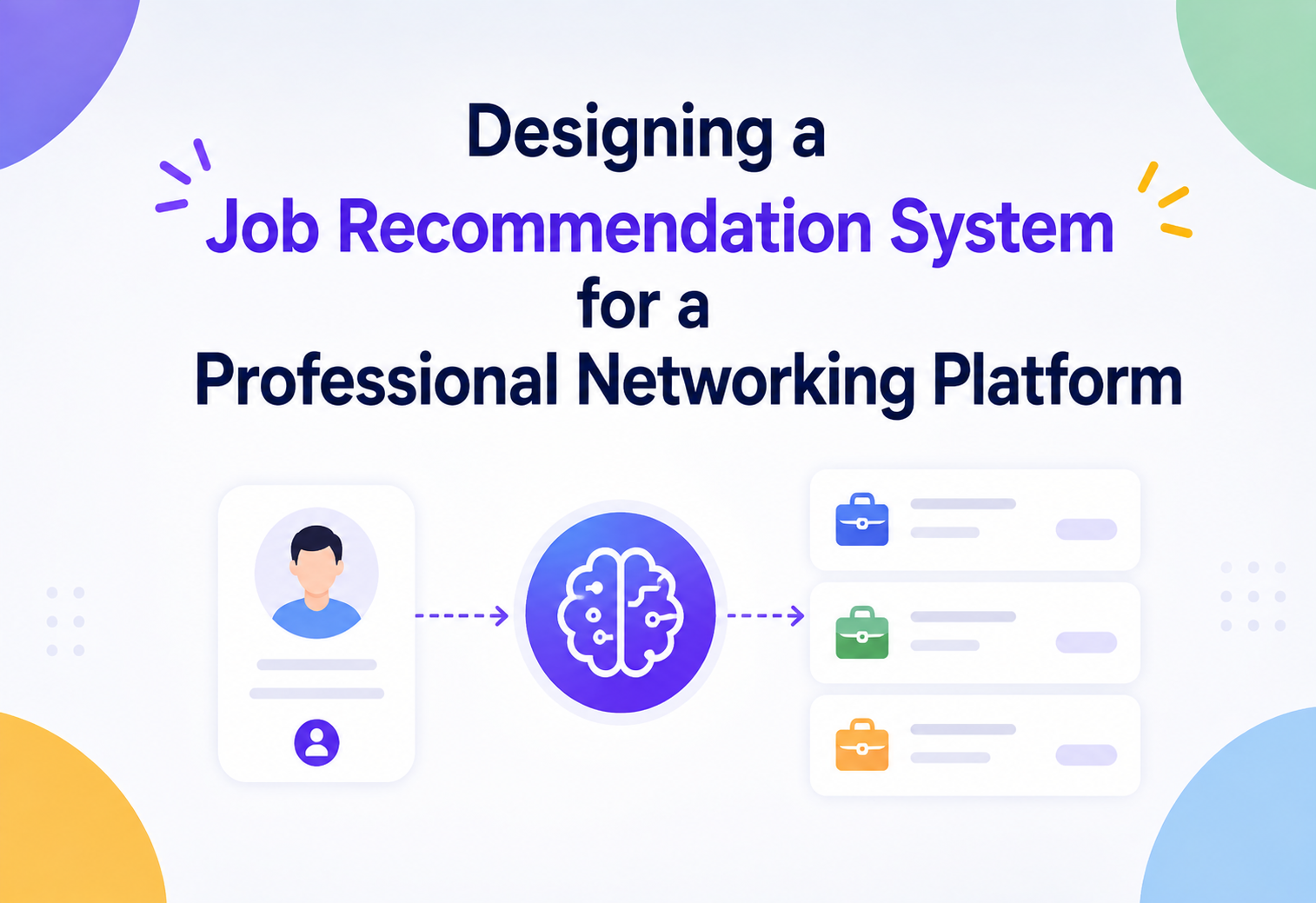
Designing a Job Recommendation System for a Professional Networking Platform
How do platforms like LinkedIn quietly figure out that you, specifically, should see this job and not that one — out of millions of postings, updated every second, for hundreds of millions of people? We are going to build that system together, brick by brick, starting from a blank whiteboard.
Introduction & History
Imagine a giant, ever-changing notice board. Every day, thousands of new job postings get pinned to it, and thousands of old ones get taken down. Millions of people walk past this board every single day. Almost nobody has the time or patience to read every single pin on that board. What everybody wants instead is: “Just show me the five or ten postings that are actually right for me.” That, in one sentence, is the entire job of a job recommendation system.
A job recommendation system is software that looks at who you are (your skills, your past jobs, your profile), what you do (what you click on, search for, apply to, ignore), and what is available (the universe of open job postings), and then produces a short, ranked list of postings that are most likely to be relevant and useful to you, right now.
1.1 A Short History of “Matching People to Work”
Before software existed, this matching was done by humans: newspaper classified ads, recruitment agencies, and word-of-mouth referrals. A recruiter with a notebook was, in a very real sense, a manual recommendation engine — they remembered “Sarah is a Java developer looking for remote work” and mentally matched her against openings they heard about.
Early job boards (Monster.com and similar sites) digitize classified ads. Search is keyword-based: you type “Java developer Bangalore” and get postings containing those exact words. There is no personalization — everyone typing the same query sees the same result.
Professional networking platforms emerge, turning résumés into structured, connected profiles. For the first time, a platform knows your work history, your skills, and your professional graph — not just a résumé PDF sitting on a server.
Collaborative filtering and content-based filtering (borrowed from e-commerce and streaming recommendation research) get applied to jobs: “People with a profile similar to yours applied to these roles” and “This posting’s required skills overlap heavily with your listed skills.”
Deep learning enters the picture. Embeddings (dense numeric fingerprints of users and jobs) replace hand-built rules. Systems start optimizing not just for clicks, but for downstream signals like actual applications and successful hires.
Modern platforms run large-scale, multi-stage recommendation pipelines: a fast candidate generation layer narrows millions of jobs down to a few hundred, and a heavier ranking layer (often a neural network) orders those few hundred precisely — all within a couple hundred milliseconds.
Think of a librarian who, instead of pointing you to the entire library, first walks you to the one shelf that matches your interest (candidate generation), and then hands you the three best books from that shelf, in the order you’d most enjoy them (ranking).
1.2 Why “Recommendation” Is Fundamentally Different From “Search”
It helps, early on, to draw a hard line between two things people often confuse: search and recommendation. When a user types “product manager remote” into a search box, they are telling the system exactly what they want, in their own words. The system’s job is simply to find postings that match those words well, and perhaps rank by recency or relevance to the query. This is a pull interaction — the user pulls information out of the system by asking a direct question.
A recommendation system solves a much harder, subtler problem: the user has not typed anything at all. They simply opened an app, and the system must proactively decide, from everything it knows about them, what they would want to see. This is a push interaction. There is no explicit query to match against — only an accumulated, evolving understanding of a person, which has to be inferred from scattered signals: a résumé filled in two years ago, a handful of recent searches, a few postings clicked and quickly abandoned, a handful of new connections at a particular company. Recommendation is, in a sense, search where the query itself has to be invented by the system before any matching can even begin.
This distinction matters enormously for system design, because it changes where the hard engineering problems live. In search, the hard problem is usually indexing and query matching (inverted indexes, tokenization, relevance scoring against an explicit query). In recommendation, the hard problem is representation — how do you compress “who this person is, professionally” into something a machine can compare against “what this job posting represents,” at a scale of hundreds of millions of comparisons per second? That representation problem is what the rest of this document is really about.
- “Why can’t we just use a simple SQL query with keyword search for job recommendations?”
- “What’s the difference between a job search system and a job recommendation system?”
- “If a user has an empty profile but has typed several job search queries, would you call that search behavior or recommendation input? How would you use it?”
Problem & Motivation
Let’s define the problem precisely, the way we would in a design interview, before touching any architecture.
2.1 The Problem Statement
Given a user’s profile (skills, experience, education, location) and their behavioral activity (searches, clicks, saves, applications, connections), recommend a ranked list of job postings from a large, constantly changing pool, such that the recommendations are relevant, fresh, diverse, and delivered within a strict latency budget — at the scale of hundreds of millions of users.
2.2 Why Is This Hard? (The Real Motivation)
Scale
Hundreds of millions of users, tens of millions of live job postings. You cannot score every job for every user in real time — the math simply doesn’t fit in a latency budget.
Freshness
Jobs open and close constantly. A posting filled yesterday must not show up today. Recommendations must reflect near-real-time inventory.
Cold Start
New users have no history. New job postings have no engagement data yet. The system must still say something reasonable for both.
Sparse, Noisy Signals
Most users apply to very few jobs. A “click” doesn’t always mean interest; an “ignore” doesn’t always mean disinterest.
Two-Sided Marketplace
You must satisfy job seekers and employers. Recommending only “easy” jobs helps no one if employers can’t find qualified applicants.
Fairness & Bias
The system must not systematically under-recommend jobs to people based on protected attributes, and must avoid reinforcing historical hiring biases.
A job recommendation system isn’t really solving “what job matches this résumé” — it’s solving “what job matches this résumé, in under 150 milliseconds, out of 50 million live options, while staying fresh, fair, and diverse.”
2.3 Framing the Problem as an Interviewer Would Expect
When this problem is posed in a system design interview, the strongest candidates resist the urge to jump straight to boxes and arrows. Instead, they spend the first several minutes doing exactly what we just did above: pinning down scale (how many users, how many jobs, how often does the catalog change), pinning down the latency and freshness expectations, and explicitly naming the hard sub-problems (cold start, marketplace balance, fairness) before proposing a single component. This ordering matters because it demonstrates the actual skill being tested — not “do you know what a vector database is,” but “can you reason from a fuzzy business problem down to a set of concrete, defensible engineering decisions.” Everything from this point in the document onward is the working-out of that reasoning, one layer at a time.
2.4 Business Goals Behind the Technical Goals
- Engagement: more relevant recommendations → more clicks, saves, applications.
- Marketplace health: employers get qualified applicants, so they keep posting jobs (this funds the platform).
- Retention: users who find genuinely useful job leads keep coming back to the platform, even when not actively job hunting.
- Trust: users must feel the recommendations understand them, not spam them with irrelevant postings.
2.5 Functional Requirements, Stated Precisely
Before drawing a single box on a whiteboard, it’s worth writing down, in plain sentences, exactly what the system must be able to do. This forces clarity and gives you something to check your architecture against later.
- Given a logged-in user, return a ranked list of job postings they are likely to find relevant, within a strict latency budget.
- Reflect newly posted jobs within minutes, and remove closed or filled jobs promptly so users never apply to a dead posting.
- Incorporate the user’s stated preferences (location, remote/hybrid/onsite, desired role, salary band) as hard constraints, not just soft ranking signals.
- Incorporate behavioral signals (recent searches, clicks, saves, applications, dismissals) to continuously refine relevance without requiring the user to explicitly restate their preferences.
- Support explanation of why a job was recommended (“2 of your connections work here,” “matches your listed skills”) to build user trust.
- Respect privacy settings, most critically the ability to hide job-seeking activity from a current employer.
2.6 Non-Functional Requirements — The Constraints That Actually Shape the Architecture
| Requirement | Target | Why It’s Non-Negotiable |
|---|---|---|
| Latency (p99) | < 200ms end-to-end | Users abandon a feed that feels slow, and mobile networks add unavoidable overhead on top of server time |
| Availability | 99.95%+ | The jobs feed is a flagship, daily-use feature — outages directly hurt engagement and trust |
| Freshness | New/closed jobs reflected within minutes | Recommending an already-filled job wastes the user’s time and damages employer relationships |
| Scalability | Hundreds of millions of users, tens of millions of active postings | The architecture must grow horizontally, not require constantly bigger single machines |
| Fairness | No systematic bias by protected attributes | Legal, ethical, and reputational exposure if recommendations discriminate |
Notice something important: these non-functional requirements actively conflict with each other in places. Freshness wants you to recompute constantly; latency and cost want you to cache aggressively. Scalability wants approximate, cheap methods; accuracy wants exact, expensive ones. A huge part of the “art” in this design is not picking one side of each trade-off absolutely, but choosing a defensible middle point — and being able to explain, out loud, why you chose it.
- “What metrics would you optimize for — clicks, applications, or hires? What are the trade-offs?”
- “How would you handle a brand-new user with zero activity (cold start)?”
- “Which non-functional requirement would you relax first if you had to cut scope for a first launch — latency, freshness, or fairness auditing? Why?”
Core Concepts
Before we design anything, we need shared vocabulary for the three core techniques the industry actually uses.
3.1 Recommendation Approaches, Explained Simply
1. Content-Based Filtering
What: recommend jobs whose content (title, required skills, description, seniority) is similar to the user’s profile content (skills, past titles, education).
Analogy: like recommending a restaurant because it serves the same cuisine you always order.
Beginner example: your profile lists “Python, SQL, Machine Learning” — the system shows postings requiring those exact skills.
Production example: a platform computes a text embedding of your profile and of every job description, then finds jobs whose embedding vector is close to yours in vector space.
2. Collaborative Filtering
What: recommend jobs that similar users engaged with, even if the job text doesn’t obviously match your profile.
Analogy: “people who bought this book also bought that book” — but for careers: “people with a similar career path also applied here.”
Beginner example: many users who share your job title and industry applied to a particular company’s opening; the system infers you might like it too, even if you’ve never searched that company’s name.
Production example: a matrix factorization or two-tower neural model learns latent (hidden) user and job embeddings purely from historical interaction data (clicks/applies), without needing to understand the text at all.
3. Hybrid / Learning-to-Rank
What: combine content-based signals, collaborative signals, recency, location, network effects (your connections work there), and dozens of other features into one machine-learned ranking model that outputs a single relevance score per job, per user.
Production example: this is what virtually every large-scale platform runs today — a gradient-boosted tree or deep neural ranking model trained on logged impressions and outcomes.
| Approach | Strength | Weakness |
|---|---|---|
| Content-based | Works even for cold-start jobs; explainable (“matches your skills”) | Can’t capture behavior patterns beyond text similarity |
| Collaborative | Captures subtle behavioral patterns humans wouldn’t hand-code | Cold start for new users/jobs with no interaction history |
| Hybrid / LTR | Best accuracy, combines strengths of both | Most complex to build, train, and maintain |
3.2 Two-Stage Recommendation: The Concept That Makes Scale Possible
Here is the single most important idea in this whole document. You cannot run a heavy, precise machine learning model over 50 million jobs for every single user request — the math simply won’t finish within your latency budget. So virtually every large-scale recommender splits the work into two stages:
- Stage 1 — Candidate Generation (recall): quickly narrow 50 million jobs down to a few hundred plausible candidates, using cheap, approximate methods (embeddings + nearest-neighbor search, rule-based filters like location/visa).
- Stage 2 — Ranking (precision): take those few hundred candidates and run a much heavier, much more accurate model to order them precisely, because now the model only has to score hundreds, not millions.
Stage 1 is like a librarian who quickly walks the aisles and pulls twenty books that look roughly on-topic. Stage 2 is like sitting down and actually reading the first page of each of those twenty to decide the exact best order — much more effort, but only spent on a small, promising set.
3.3 Embeddings, Explained From First Principles
The word “embedding” comes up constantly in this domain, so it’s worth building genuine intuition for it rather than treating it as jargon. An embedding is simply a list of numbers (a vector) that represents something — a word, a sentence, a user, a job posting — in such a way that similar things end up with similar numbers, and dissimilar things end up with very different numbers.
Beginner example: imagine you described every job posting using just two numbers: “how technical is this role” (0 to 1) and “how senior is this role” (0 to 1). A “Senior Backend Engineer” posting might become the pair (0.9, 0.8). A “Junior Marketing Coordinator” might become (0.1, 0.2). Suddenly, “how similar are these two jobs” becomes a simple geometry question — how close together are these two points on a 2D graph? Real embeddings do exactly this, except instead of 2 hand-picked numbers, they use hundreds of numbers, and instead of numbers a human designed, a neural network learns them automatically from data, capturing far subtler patterns than any human could hand-craft.
Software example: a job description’s text (“5+ years of experience with distributed systems, Kafka, and Java…”) is fed through a language model, which outputs, say, a 256-number vector. A user’s profile text (skills, past titles, summary) is fed through a similar model, producing another 256-number vector in the exact same numeric space. Two vectors that point in a similar direction (measured by cosine similarity — the angle between them) represent a user and a job that are professionally aligned, even if they don’t share a single identical word.
Production example: at scale, these vectors for tens of millions of jobs are precomputed once (or refreshed periodically) and stored in a specialized vector database, indexed using structures like HNSW (Hierarchical Navigable Small World graphs) that let you find the “closest” vectors to a query vector in milliseconds, without comparing against every single one of the tens of millions stored — this is exactly what makes Approximate Nearest Neighbor (ANN) search fast enough to sit in the critical serving path.

Think of embeddings like GPS coordinates for meaning. Just as two restaurants with similar coordinates are physically close and easy to walk between, two jobs (or a user and a job) with similar embeddings are “professionally close,” even if their text descriptions use completely different words.
3.4 Explicit vs. Implicit Signals
Not all data about a user is equally trustworthy or equally strong. It helps to separate signals into two buckets.
Explicit Signals
Things the user directly told the platform: listed skills, stated job preferences, desired salary, “not interested in this role” feedback. Strong, unambiguous, but sparse — most users don’t fill in every field.
Implicit Signals
Things inferred from behavior: which postings they lingered on, which they scrolled past instantly, which they saved but never applied to. Abundant, but noisier — a click doesn’t always mean genuine interest.
A well-designed system blends both: explicit signals as strong priors (especially useful for cold-start users), and implicit behavioral signals as the continuously updating, high-volume stream that keeps recommendations feeling responsive to what a user actually does, not just what they once typed into a form.
3.5 Feature Engineering: Turning Raw Signals Into Model-Ready Inputs
Neither embeddings nor raw event logs are, by themselves, exactly what a ranking model consumes — there’s a translation step in between called feature engineering, and it’s worth understanding why it matters so much in practice. A raw fact like “user clicked job X three days ago” isn’t directly useful to a model; it needs to be transformed into a well-shaped numeric signal, such as “number of clicks on jobs in this same job family within the last 14 days,” or “days since the user’s most recent application.” These engineered features encode domain knowledge — a system designer’s understanding of what kinds of patterns actually predict relevance — into a form the model can learn from efficiently.
Good feature engineering in this domain typically spans several families: profile features (years of experience, listed skills, education level), behavioral features (recency and frequency of searches, clicks, saves, applications, broken down by job category), graph features (connections at the employer, shared alumni networks, mutual connections who hold similar titles), job features (posting age, number of applicants so far, required skill count, salary transparency), and interaction features that explicitly combine a user attribute with a job attribute (skill-overlap percentage, location distance, seniority-level match). It’s this last family — interaction features — that often carries the most predictive power, precisely because relevance is fundamentally about the fit between a person and a job, not either one considered alone.
3.6 How You Actually Know if the Recommendations Are Good: Offline Evaluation Metrics
Before ever showing a new model to real users, teams evaluate it offline against historical logs, using metrics purpose-built for ranked lists rather than simple accuracy. Precision@K asks: of the top K jobs shown, how many were ones the user actually engaged with? Recall@K asks: of all the jobs the user eventually engaged with, how many appeared somewhere in the top K? NDCG (Normalized Discounted Cumulative Gain) goes further, rewarding a model more for placing a truly relevant job at position 1 than at position 10, capturing the intuition that where in the list something appears matters, not just whether it appears at all. These offline metrics are cheap and fast to compute against historical data, letting a team iterate on model changes quickly, before ever spending the time and risk of a live online A/B test.
Imagine handing someone a stack of ten job postings. Getting the single best one onto the very top of the stack is worth far more to them than burying it at position eight, even though technically “it’s in there somewhere” either way. NDCG is simply a formal way of rewarding a model for getting that ordering right, not just for including the right items somewhere.
- “Why do we need two stages instead of one big model scoring everything?”
- “What happens if candidate generation misses a genuinely great job for a user? How would you detect that?”
- “How would you weigh an explicit ‘not interested’ signal against a strong implicit signal like repeated clicks on similar jobs?”
Architecture & Components
Now let’s put the whole system on the whiteboard. Every box below is a real, independently scalable component — and every box is explicitly labeled with what it is, so nothing is left implicit. Before looking at the diagram, it helps to walk through the reasoning that leads to this specific shape, rather than treating it as a fixed answer to memorize.
We start at the edge, because every request, regardless of what it eventually does, must first arrive somewhere. A Load Balancer is the natural first stop: it exists purely to spread incoming traffic evenly across many identical backend instances and to detect and route around unhealthy ones, so no single machine becomes a bottleneck or single point of failure. Just behind it sits an API Gateway, which centralizes cross-cutting concerns — authentication, rate limiting, request validation — that would otherwise need to be reimplemented, inconsistently, inside every single backend service.
Once a request is authenticated and past the gateway, it needs a component whose entire job is to coordinate the rest of the work — we call this the Feed Orchestrator. Rather than have the client talk to five different backend services directly (which would leak internal architecture to the client and make future refactoring painful), the orchestrator acts as the single point of coordination, fanning out to whichever downstream services it needs and assembling one coherent response.
From here, the design branches into two parallel concerns that must both be satisfied before a response can be built: who is this user (Profile Service, Activity Service) and what’s out there for them (Candidate Generation, backed by the Vector Database). Finally, once we have a manageable shortlist of candidate jobs, a dedicated Ranking Service applies the heaviest, most precise computation — a machine learning model — to exactly that small shortlist, never to the full universe of jobs, which is what keeps the whole pipeline fast despite doing genuinely sophisticated modeling.
Underneath all of this sits the data backbone: a durable event stream (Kafka) capturing every user action as it happens, a stream processor turning that raw event stream into ready-to-use features, and an offline training pipeline that periodically mines the accumulated history to produce better models over time. None of these components exist in isolation — each one earns its place in the diagram by solving a specific, named problem introduced back in Sections 2 and 3.
4.1 Component Reference (What Every Box in the Diagram Actually Does)
Load Balancer
Layer-7 load balancer (e.g., an Application Load Balancer or Envoy) distributes incoming HTTPS traffic across many API Gateway instances, does health checks, and terminates TLS. Prevents any single server from being overwhelmed.
API Gateway
Single entry point for all client requests. Handles authentication (JWT/OAuth), request throttling/rate limiting, request routing to the right backend service, and basic request validation, so internal services don’t each reimplement this.
Feed Orchestrator Service
The “conductor.” Receives “give me my job feed” requests, fans out calls to Profile, Activity, Candidate Generation, and Ranking services in parallel, assembles the final response, and applies business rules (e.g., diversity, de-duplication).
Profile Service
Owns and serves structured user profile data: skills, past titles, education, location, preferences. Backed by a distributed database optimized for fast key-based reads.
Activity Service
Records and serves user behavioral signals — searches, clicks, saves, applies, dismissals — used both for real-time personalization and for training data.
Candidate Generation Service
Given a user embedding, performs Approximate Nearest Neighbor (ANN) search against a vector index of job embeddings to retrieve a few hundred plausible jobs in single-digit milliseconds, combined with hard filters (location, visa status, already-applied).
Vector Database / ANN Index
Stores dense embedding vectors for every active job posting (and often user embeddings too), indexed using structures like HNSW or IVF for fast similarity search across tens of millions of vectors.
Feature Store
A centralized system (online + offline) that serves precomputed features (e.g., “user’s average job-search recency,” “job’s application rate this week”) consistently to both the ranking model at serving time and the training pipeline offline — avoiding train/serve skew.
Ranking Service
Hosts the trained ranking model (e.g., a gradient-boosted tree or deep neural network) behind a low-latency inference server. Takes the few hundred candidates plus their features and outputs a precise relevance score for each.
Model Registry
Versioned storage for trained models, enabling safe rollout, rollback, and A/B testing of new ranking models without redeploying application code.
Redis Cache
In-memory cache storing recently computed feed results and hot features, keyed by user ID, with a short TTL — dramatically reduces load on downstream services for repeated requests (e.g., user refreshing the app).
Kafka Event Stream
Durable, ordered, high-throughput message log that ingests every user interaction event in near real time, decoupling producers (client apps) from consumers (stream processors, training pipelines).
Stream Processor (Flink/Spark Streaming)
Consumes the Kafka event stream continuously, computes rolling/windowed features (e.g., “clicks in the last hour”), and writes them into the Feature Store in near real time.
Job Postings DB
Sharded relational (or document) database that is the system of record for every job posting: title, description, requirements, employer, status (open/closed).
Job Indexer
Watches for new/updated/closed job postings and pushes updates into both the Search Index and the Vector Database, keeping recommendations fresh within seconds to minutes.
Search Index
Elasticsearch/OpenSearch. Powers keyword-based job search (distinct from, but complementary to, embedding-based recommendation) and supports hard filters like “remote only” or “posted in last 24 hours.”
Offline Training Pipeline
Batch jobs (commonly on Spark) that periodically retrain the ranking and embedding models using historical profile, job, and activity data, then publish new model versions to the Model Registry.
- “Why do we need both a Search Index and a Vector Database — aren’t they redundant?”
- “Where exactly would you put caching, and what would you cache — the raw candidates, the final ranked list, or both?”
- “What happens to this diagram if the Ranking Service goes down — do users see nothing?”
Internal Working
Let’s trace exactly what happens, component by component, the instant a user opens their “Jobs For You” tab.
5.1 Step-by-Step, in Plain English
- Request enters through the Load Balancer, which picks a healthy API Gateway instance to handle it.
- The API Gateway authenticates the user (verifies their session token) and checks they haven’t exceeded their rate limit.
- The Feed Orchestrator first checks Redis — if this user requested their feed 30 seconds ago and nothing material has changed, we simply return the cached list. This alone removes enormous load from the rest of the pipeline.
- On a cache miss, the orchestrator asks the Candidate Generation Service for a shortlist. That service converts the user’s profile + recent activity into a numeric embedding vector, then performs an Approximate Nearest Neighbor search against the Vector Database to find the ~500 closest job vectors — this takes single-digit milliseconds even across tens of millions of jobs, because ANN indexes trade a tiny bit of accuracy for massive speed.
- Hard filters apply at this stage too: remove jobs the user already applied to, jobs outside their stated location/visa constraints, and jobs that have since closed.
- Features are fetched from the Feature Store for exactly this (user, candidate-jobs) pair — things like “does a 1st-degree connection work there,” “skill overlap percentage,” “job posting age,” “user’s historical application rate for this job function.”
- The Ranking Service scores every candidate using the trained model, producing a precise relevance score per job.
- The orchestrator applies business logic: diversity rules (don’t show ten postings from the same company back-to-back), de-duplication, and final ordering.
- The result is cached briefly and returned to the user.
ANN search is approximate — it might miss the single mathematically-best job in exchange for being thousands of times faster than an exact nearest-neighbor scan. This trade-off (index type, e.g. HNSW vs IVF-PQ) directly affects recall, and is a deliberate, tunable engineering choice, not a bug.
5.2 Inside the Ranking Service: What the Model Actually Computes
It’s worth pulling back the curtain on what “score this candidate job” actually means computationally, since this is often glossed over. For each (user, job) pair among the few hundred candidates, the Ranking Service assembles a feature vector — a list of numbers describing the pairing. This typically includes: content-similarity features (embedding cosine similarity between user and job), graph features (number of first-degree connections at the employer, whether anyone in the user’s network has this exact title), behavioral features (has this user historically applied to similar roles, how recently did they last engage with this job function), and job-quality features (how many applicants so far, how long it’s been posted, whether the employer has a strong response-rate history).
This feature vector is fed into the trained model — commonly a gradient-boosted decision tree ensemble (like XGBoost or LightGBM) for interpretability and speed, or a deep neural network (often a two-tower architecture, where one tower encodes the user and one encodes the job, with a final layer combining them) for capturing more complex, non-linear interactions. The output is a single number: a relevance score, typically between 0 and 1, representing the model’s estimate of how likely this user is to engage positively with this particular job.
Crucially, this scoring is batched — rather than invoking the model 500 separate times (once per candidate), the Ranking Service assembles all 500 feature vectors into a single matrix and performs one batched inference call, which is dramatically more efficient on modern hardware (CPU vectorization or GPU parallelism) than many small calls.
5.3 Why Parallel Fan-Out Matters So Much Here
Look again at the sequence diagram in Fig 2. Notice that fetching the user’s profile, fetching their recent activity, and running candidate generation are all logically independent of each other — none of them needs the output of the others to begin. A naive implementation might call them one after another, sequentially, multiplying their individual latencies into one large total. A well-designed Feed Orchestrator instead issues these calls concurrently (using asynchronous I/O or parallel threads) and waits for all of them to complete before proceeding, meaning the total added latency is roughly the slowest of the parallel calls, not the sum of all of them. This single implementation detail — fan-out in parallel rather than in sequence — is often the difference between a feed that loads in 90ms and one that loads in 300ms, using the exact same set of backend services.
- “Walk me through what happens end-to-end when a user opens the jobs tab — where could latency creep in?”
- “How would you keep the Feature Store consistent between what the model saw during training and what it sees at serving time?”
- “Why batch the ranking model’s inference calls instead of scoring each candidate job individually?”
Data Flow & Lifecycle
Two very different data flows power this system, and it’s important to keep them mentally separate: the online (serving) path, which must be fast, and the offline (training) path, which can be slow but must be thorough.
6.1 Lifecycle of a Single Job Posting
Employer submits a posting → written to the Job Postings DB → Job Indexer picks it up → indexed into both the Search Index and the Vector Database (an embedding is computed from its text) within seconds.
The posting is now eligible to appear in candidate generation and ranking for any matching user.
Every impression, click, save, and application against this posting is logged as an event to Kafka, updating its “engagement features” (e.g., application rate) in near real time via the stream processor.
Employer closes it (or it auto-expires) → status flips in the Job Postings DB → indexer removes it from the Search Index and Vector Database so it instantly stops being recommended.
Historical data about the posting (and its outcomes) is retained in the data lake, feeding future model training even after the posting itself is gone.
6.2 Lifecycle of a Single User Interaction
Click on a job → event emitted to Kafka → stream processor updates rolling features (“user clicked 3 data-science jobs in the last hour”) → feature store updated → next request for this user’s feed reflects the freshly updated signal → periodically, this same click also lands in the data lake as training data for the next model retrain.
6.3 Batch vs. Streaming: Why This System Needs Both
A recurring question in any data-intensive system is whether to process data in batches (large chunks, on a schedule — hourly, daily) or as a stream (processing each event individually, the instant it arrives). This architecture deliberately uses both, because they solve different problems well.
Streaming (via the Kafka + stream processor pipeline) is essential for anything that needs to feel immediately responsive: a user clicking a job should be reflected in their next feed request seconds later, not tomorrow. Batch processing (via the offline Spark-based training pipeline) is appropriate — and actually preferable — for anything that benefits from seeing the full, stable picture: training a model on the last 90 days of data produces a more robust model than trying to retrain it continuously on every single new data point, which would be both computationally wasteful and statistically noisy (each individual click is a very weak, high-variance training signal on its own).
A useful mental model: streaming keeps the system reactive; batch keeps the system smart. The stream processor updates lightweight, immediate features (“clicked 3 similar jobs in the last hour”); the batch pipeline periodically re-learns the deeper, more stable patterns (“users with this career trajectory tend to respond well to this category of role”), and pushes an updated model into the Model Registry for the serving path to pick up.
6.4 The Feedback Loop, Made Explicit
Every recommendation shown to a user becomes, eventually, a new row of training data for the next model. This creates a loop: model recommends → user reacts (click/apply/ignore) → reaction is logged → next model trains on that reaction → new model recommends differently. This loop is powerful (it’s literally how the system learns and improves) but also dangerous if left unchecked, because the model only ever observes outcomes for jobs it already chose to show. It never learns what would have happened for a job it never surfaced in the first place — a well-known issue sometimes called exposure bias. The standard mitigation, introduced briefly in Section 3 and expanded on in Section 14, is to deliberately reserve a small slice of impressions for exploration — occasionally surfacing a promising-but-unproven job slightly higher than the model alone would rank it, purely to gather unbiased feedback that keeps future training data honest.
- “How fresh does a user’s activity need to be before it affects their next recommendation? What would you trade off to make it fresher?”
- “How do you avoid a feedback loop where the model only ever recommends what it already recommended before?”
- “Why not just retrain the model continuously on every single new click, in real time?”
Databases, Caching & Load Balancing
7.1 Choosing the Right Store for the Right Job
| Data | Store Type | Why |
|---|---|---|
| User profiles | Distributed relational (sharded Postgres/MySQL) or wide-column NoSQL | Structured, frequently read by primary key, moderate write volume |
| Job postings | Sharded relational DB | Structured with relationships (employer → posting), transactional writes on create/close |
| Job/user embeddings | Vector database (e.g., HNSW-based ANN index) | Needs approximate nearest-neighbor search across tens of millions of high-dimensional vectors, sub-10ms |
| Full-text job search | Elasticsearch/OpenSearch | Inverted index built for keyword and filter-based search, not similarity search |
| Real-time features | Online feature store (Redis/key-value backed) | Millisecond reads keyed by user/job ID, written continuously by the stream processor |
| Historical activity/training data | Data lake (columnar, e.g. Parquet on object storage) | Massive volume, append-only, optimized for batch scans not point lookups |
| Hot feed results | Redis cache (in-memory) | Sub-millisecond reads for repeated requests within a short TTL window |
7.2 Caching Strategy
- Feed-level cache: cache the fully ranked list per user for a few minutes — most users don’t refresh the feed constantly, so this alone avoids re-running the whole pipeline on every request.
- Feature-level cache: cache computed features (not just final results) so a cache miss on the feed doesn’t force recomputation of everything from scratch.
- Cache invalidation: use short TTLs (time-to-live) rather than explicit invalidation for feed results, since job freshness only needs “eventually consistent within minutes,” not instant consistency — invalidating on every job change would be far too chatty at this scale.
The cache is like keeping a photocopy of your last grocery list on the fridge — if you’re heading to the store again five minutes later, you grab the photocopy instead of re-thinking your whole meal plan from scratch.
7.3 Load Balancing in Depth
A single Load Balancer sits in front of the API Gateway fleet and typically uses a Layer-7 (HTTP-aware) strategy so it can route based on path or header, do TLS termination, and run active health checks (removing an unhealthy instance from rotation automatically). Internally, service-to-service calls (e.g., Feed Orchestrator → Ranking Service) commonly use a lighter client-side or sidecar load balancer (as in a service mesh) using round-robin or least-connections strategies.
7.4 SQL vs. NoSQL, and Where the CAP Theorem Shows Up
The Job Postings DB and Profile Service illustrate a classic decision every system designer eventually faces: relational (SQL) versus non-relational (NoSQL) storage. Relational databases give strong consistency guarantees and rich querying (joins, transactions) but traditionally scale writes less gracefully without sharding. NoSQL wide-column or document stores scale horizontally far more naturally but often relax consistency guarantees to do so.
This is where the CAP theorem becomes concretely relevant, not just theoretical. CAP states that a distributed data store can only guarantee two of three properties at once during a network partition: Consistency (every read sees the latest write), Availability (every request gets a response, even if it might be stale), and Partition tolerance (the system keeps working despite network splits between nodes). Since partition tolerance is essentially mandatory for any distributed system running across multiple data centers, the real choice in practice is between consistency and availability during a partition.
For the Job Postings DB, we lean toward availability with eventual consistency — if a job’s “closed” status takes a few extra seconds to propagate to every replica during a network hiccup, that’s a tolerable, minor annoyance, not a catastrophe. For something like a payment or billing record tied to job postings (an employer’s ad spend, for instance), we’d lean the opposite way, favoring strict consistency even at some cost to availability, because an incorrect balance is a much more serious problem than a few seconds of staleness.
7.5 Handling Hot Keys and Skewed Access Patterns
Not all users or jobs receive equal traffic. A newly viral job posting, or a heavily-followed influential user, can receive disproportionate read traffic — a “hot key” — that can overwhelm a single database shard or cache node even while the overall system has plenty of spare capacity elsewhere. Common mitigations include: replicating especially hot data across multiple cache nodes rather than pinning it to one; adding a short random jitter to cache TTLs so many clients don’t all expire and recompute the same hot key simultaneously (avoiding a “thundering herd”); and, for extreme cases, a local in-process cache layer in front of the shared Redis cache, absorbing the very hottest reads before they ever leave a single instance.
- “Why use a vector database in addition to a traditional relational database — why not just store embeddings as a column?”
- “How would you handle a ‘hot key’ problem if a celebrity-like user or an extremely popular job posting gets disproportionate traffic?”
- “Where in this system would you accept eventual consistency, and where would you insist on strong consistency? Why?”
APIs & Microservices
8.1 Representative Public API
GET /v1/jobs/recommendations?userId=8842&limit=20&cursor=eyJvZmZzZXQ...
Authorization: Bearer <jwt>

200 OK
{
  "userId": "8842",
  "generatedAt": "2026-07-28T09:15:32Z",
  "jobs": [
    {
      "jobId": "job_991238",
      "title": "Senior Backend Engineer",
      "company": "Acme Corp",
      "location": "Bengaluru, India (Hybrid)",
      "relevanceScore": 0.912,
      "matchReasons": ["Skill overlap: Java, Kafka", "2 connections work here"]
    }
  ],
  "nextCursor": "eyJvZmZzZXQ..."
}
8.2 Core Internal Service Contracts (Java)
public interface RankingService {
    // Scores each candidate job for the given user, returns descending order
    List<ScoredJob> rankCandidates(String userId, List<String> candidateJobIds);
}

public class ScoredJob {
    private final String jobId;
    private final double relevanceScore;
    private final Map<String, Double> featureContributions; // for explainability

    public ScoredJob(String jobId, double relevanceScore,
                     Map<String, Double> featureContributions) {
        this.jobId = jobId;
        this.relevanceScore = relevanceScore;
        this.featureContributions = featureContributions;
    }
    // getters omitted for brevity
}public class CandidateGenerationService {
private final VectorIndexClient vectorIndex;
private final JobFilterService filterService;
public List<String> generateCandidates(String userId, int topK) {
float[] userEmbedding = this.fetchUserEmbedding(userId);
// Approximate Nearest Neighbor search against job embeddings
List<String> rawCandidates =
vectorIndex.query(userEmbedding, topK * 2); // over-fetch before filtering
// Apply hard filters: location, visa, already-applied, closed jobs
return filterService.applyHardFilters(userId, rawCandidates)
.stream()
.limit(topK)
.collect(Collectors.toList());
}
}8.3 Microservice Boundaries — Why Split It Up This Way?
- Independent scaling: the Ranking Service is CPU/GPU-heavy and needs different scaling rules than the lightweight Profile Service.
- Independent deployment: data scientists can ship a new ranking model without redeploying the entire orchestrator.
- Failure isolation: if the Ranking Service degrades, the orchestrator can fall back to a simpler ordering (e.g., recency-based) instead of taking down the whole feed.
- Team ownership: ML teams own Candidate Gen/Ranking; platform teams own Profile/Activity/Gateway — clean API boundaries let them move independently (Conway’s Law in action).
8.4 API Versioning Strategy, Concretely
Notice the API path in the example above begins with /v1/. This is not decoration — it’s a deliberate contract. Mobile apps, in particular, can lag far behind the latest backend deployment, since users don’t always update apps immediately (or at all). If the response schema changes in a way that breaks older clients (renaming a field, removing one an old app depends on), those users would see crashes or broken feeds until they update — often for weeks or months. Versioning the API path allows the backend to introduce a new /v2/ endpoint with a changed schema while continuing to serve /v1/ unchanged for as long as meaningfully-sized old client versions remain in the wild, only deprecating it once usage drops below a defined threshold.
A subtler, complementary practice is designing response schemas to be additive by default — new fields can be added freely (old clients simply ignore fields they don’t recognize), but existing fields should never change type or meaning within the same version. This single discipline avoids the need for a new API version far more often than teams expect.
8.5 Synchronous Versus Asynchronous Service Communication
Not every interaction between these services needs to be a synchronous, blocking call awaiting an immediate response. The request-time path (Gateway → Orchestrator → Candidate Gen → Ranking) is necessarily synchronous, because the client is actively waiting for an answer. But plenty of the system’s internal machinery is deliberately asynchronous: when a user clicks a job, the Activity Service doesn’t need to synchronously wait for the stream processor to finish updating features before returning success to the client — it publishes an event to Kafka and returns immediately, letting the stream processor consume and process that event on its own schedule, decoupled entirely from the user-facing request. This asynchronous decoupling is what allows the real-time activity pipeline to absorb traffic spikes gracefully, since Kafka acts as a durable buffer between fast producers and potentially slower consumers.
- “Would you expose the Ranking Service directly to clients, or always go through an orchestrator? Why?”
- “How would you version this API so mobile apps on an older version don’t break when you change the response schema?”
- “Why is logging a user’s click event asynchronous, while fetching their ranked feed is synchronous?”
Performance & Scalability
9.1 Latency Budget Breakdown
| Stage | Budget |
|---|---|
| Gateway + auth | ~10 ms |
| ANN candidate search | ~15 ms |
| Feature fetch | ~10 ms |
| Ranking model inference | ~40 ms |
| Aggregation + business rules | ~10 ms |
That totals roughly 85ms of compute, leaving headroom within a ~150ms end-to-end target even after network overhead — but only because Stage 1 (candidate generation) drastically shrinks the problem before Stage 2 (ranking) has to do heavy lifting.
9.2 Horizontal Scaling Techniques
- Stateless services: the API Gateway, Feed Orchestrator, and Ranking Service are all stateless — any instance can handle any request, so you scale by simply adding more instances behind the load balancer.
- Sharding the Job Postings DB: shard by job ID hash (or by employer ID) so writes and reads distribute across many database nodes instead of one.
- Sharding the Vector Database: partition the ANN index (e.g., by geography or job category) so each shard holds a manageable subset of vectors, and search fans out across shards in parallel.
- Batching model inference: the Ranking Service scores hundreds of candidates in one batched GPU/CPU call rather than one-by-one, dramatically improving throughput per request.
- Read replicas: the Profile Service reads from replicas for the (far more common) read path, reserving the primary for writes.
9.3 Applying Little’s Law to Size the Ranking Service Fleet
Little’s Law states: L = λ × W — the average number of requests in the system (L) equals the arrival rate (λ) multiplied by the average time each request spends in the system (W). If the Ranking Service receives 20,000 requests/second and each takes 40ms (0.04s) to process, then on average L = 20,000 × 0.04 = 800 requests are “in flight” at any instant — telling you roughly how many concurrent inference slots (threads/GPU batches) you need provisioned to avoid queuing delay.
If a coffee shop serves 1 customer every 2 minutes on average and gets 1 new customer every 2 minutes, there’s always roughly 1 customer being served. Speed up service or add baristas, and the queue (and average wait) shrinks even without more customers walking in.
9.4 Vertical vs. Horizontal Scaling, and Why This System Leans Almost Entirely Horizontal
It’s worth explicitly naming the two ways any system can grow. Vertical scaling means making a single machine bigger — more CPU cores, more RAM, a faster disk. Horizontal scaling means adding more machines and spreading the work across them. Vertical scaling is simpler (no distributed coordination needed) but hits a hard ceiling — there is only so big a single machine can get, and at some point the cost curve becomes brutal. Horizontal scaling has no such ceiling, but it demands that services be stateless (or that state be carefully partitioned), so that any of many identical instances can handle any incoming request.
This is precisely why every compute-heavy service in this architecture — the API Gateway, the Feed Orchestrator, the Candidate Generation Service, the Ranking Service — is designed to be stateless. None of them hold onto per-user session data between requests; instead, all persistent state lives in the databases, caches, and the feature store. This single design choice is what allows the platform to absorb a sudden traffic spike (say, a viral news story driving a surge of job seekers) simply by spinning up more container instances behind the load balancer, rather than needing to somehow make existing machines more powerful on the fly.
9.5 Capacity Planning Walkthrough
Suppose product analytics tells us the platform expects 500 million daily active users, each opening the jobs feed an average of 3 times per day. That’s 1.5 billion feed requests per day, or roughly 17,360 requests per second on average — but averages hide the real danger, which is peak load. If traffic during peak hours (say, weekday mornings) is 4 times the daily average, peak throughput could reach roughly 70,000 requests per second. Using our earlier latency budget of about 85ms of compute per request, and applying Little’s Law, we’d need capacity for roughly 70,000 × 0.085 ≈ 5,950 requests “in flight” concurrently across the fleet at peak — a number that directly informs how many Ranking Service and Candidate Generation Service instances (and, for the Ranking Service, how many GPU-backed inference workers) need to be provisioned, with headroom for safety margin and for one availability zone failing over into others.
9.6 Reducing Load Before It Ever Reaches the Expensive Tiers
- Client-side debouncing: don’t fire a new feed request every time the user scrolls slightly — batch and debounce requests from the client.
- Pagination with cursors: return the feed in pages (e.g., 20 jobs at a time) rather than computing and transmitting a giant list upfront, so ranking work for page 2 only happens if the user actually scrolls that far.
- Precomputation during off-peak hours: for less time-sensitive users (e.g., users who log in rarely), precompute and cache a full day’s feed overnight when infrastructure is under-utilized, rather than computing it live during a traffic peak.
- “If p99 latency spikes under load, where would you look first — the ANN index, the feature store, or the ranking model?”
- “How would you scale the vector index as the job catalog grows from 50 million to 500 million postings?”
- “Walk me through how you’d estimate the number of Ranking Service instances needed for a given traffic forecast.”
HA & Reliability
10.1 Graceful Degradation, Not Total Failure
The single most important reliability principle here: a slightly worse job feed is infinitely better than no job feed. Every stage of the pipeline needs a fallback.
✓ Fallback Ladder (Best → Acceptable)
- Full personalized ranking (normal path)
- Cached ranked list (a few minutes stale)
- Candidate list without fine ranking (recency-sorted)
- Popular/trending jobs in user’s location (fully generic)
✗ What NOT to Do
- Return a hard error/blank screen when Ranking Service times out
- Let one slow downstream call block the entire response indefinitely
- Retry aggressively without backoff, worsening an already-struggling service
10.2 Key Reliability Patterns Applied Here
- Circuit breaker: the Feed Orchestrator wraps its call to the Ranking Service in a circuit breaker — after enough consecutive failures/timeouts, it “opens” and immediately falls back to cached/candidate-only results instead of waiting on a doomed call.
- Timeouts + retries with jitter: every downstream call has a strict timeout (e.g., 50ms for ranking), and any retry uses randomized jitter to avoid synchronized retry storms across thousands of orchestrator instances.
- Bulkheads: the thread pool used to call the Ranking Service is isolated from the pool used to call the Profile Service, so a slow ranking model can’t starve unrelated calls of threads.
- Multi-AZ / multi-region deployment: stateless services and databases replicate across availability zones so a single data-center failure doesn’t take the platform down.
- Replication for the Vector DB and Job Postings DB: leader-follower replication so a leader failure promotes a follower with minimal data loss.
Incoming request → circuit-breaker check on Ranking Service: if healthy (closed), take the full ML ranking path; if failing (open), skip straight to the fallback (cached list or recency-sorted candidates). Either branch feeds the same response back to the client, so the user never sees a hard failure — only, at worst, a slightly less personalized feed.
10.3 Replication and Consensus, Briefly
When we say the Job Postings DB or Vector Database “replicates,” it’s worth being precise about what that means and what it costs. In a typical leader-follower replication setup, one node (the leader) accepts all writes and streams those changes to one or more follower nodes, which serve read traffic and stand ready to be promoted if the leader fails. This works well and is simple to reason about, but it does introduce a brief window of risk: if the leader fails before a write has been replicated to any follower, that write can be lost.
For data where this is unacceptable — critical billing or transactional records tied to job postings, for instance — systems often use a consensus protocol (such as Raft or Paxos) to ensure a write is only acknowledged once a majority of nodes agree they’ve received it, trading a small amount of write latency for a much stronger durability guarantee. For the bulk of this system’s data — job listings, embeddings, activity logs — simple leader-follower replication with asynchronous followers is an accepted, pragmatic trade-off, because losing a few seconds of the very latest writes during a rare leader failure is a far smaller cost than the added latency and complexity of full consensus on every write.
10.4 Disaster Recovery and Backup Strategy
Beyond day-to-day replication, the system needs a plan for genuinely catastrophic scenarios — an entire region becoming unavailable, or a serious data corruption bug silently propagating writes. This typically means: point-in-time backups of the Job Postings DB and Profile Service databases, retained long enough to recover from a corruption discovered days later, not just minutes; regular, automated restore drills (a backup nobody has ever successfully restored from is not a real backup); and a documented, tested failover runbook for promoting a secondary region to primary, including how DNS and load balancer configuration would be updated to redirect traffic during such an event.
- “What’s your fallback if the Vector Database cluster is completely unreachable?”
- “How would you design retries between the Feed Orchestrator and Ranking Service to avoid a retry storm during a partial outage?”
- “What’s the difference between leader-follower replication and a consensus protocol like Raft, and when would you reach for the stronger, more expensive option?”
Security
- Authentication & authorization: every request carries a signed JWT validated at the API Gateway; the Feed Orchestrator never trusts a raw user ID from the client without this verification.
- Least privilege between services: the Ranking Service can read features but has no write access to the Profile Service’s database; service-to-service auth uses mutual TLS (mTLS) within the internal network.
- Rate limiting at the gateway: prevents scraping of job data or profile-probing at scale (e.g., someone trying to enumerate which users are actively job-hunting, a sensitive signal for current employers to know).
- PII protection: activity logs and training data are scrubbed/pseudonymized where possible; access to raw profile/activity data is restricted and audited, since “who is job hunting” is highly sensitive information.
- Encryption: TLS in transit everywhere (client↔gateway and service↔service); encryption at rest for the Profile DB, Job Postings DB, and data lake.
- Employer-side protections: validate and moderate job postings against injected malicious content (XSS in job descriptions) before they are indexed and rendered to job seekers.
- Privacy controls: respect a user’s “don’t show my activity to my current employer” setting — this must be enforced as a hard filter, not just a ranking preference, since a leak here has real career consequences for the user.
Unlike a shopping recommender, leaking “this user is looking at job postings” to the wrong party (e.g., their current employer) can cost someone their job. Privacy-by-design isn’t optional here — it’s core to the product.
11.1 Defense in Depth, Applied to This Specific System
Security here isn’t a single control bolted on at the edge — it’s layered, so that if any single safeguard fails, others still hold the line. At the outermost layer, the Load Balancer terminates TLS and can absorb basic volumetric attacks. Just inside that, the API Gateway enforces authentication and rate limiting, so an attacker who somehow bypasses the outer layer still hits a wall before reaching any real data. Inside the internal network, service-to-service calls use mutual TLS so that even a compromised internal service can’t silently impersonate another. And at the very core, the data stores themselves enforce field-level access controls, so that even a service with legitimate network access can only read the specific fields its function actually requires — the Ranking Service, for instance, has no business reading a user’s raw contact details, only their skill and activity features.
This layered approach matters because in a system built from many independently-deployed microservices, the classic advice of “just have one strong perimeter” doesn’t hold — an internal service, once compromised, effectively sits behind the perimeter already. Defense in depth assumes any single layer can fail and asks what happens next.

11.2 Regulatory Compliance Considerations
A platform holding detailed professional histories on hundreds of millions of people across many countries operates under serious regulatory obligations, most notably data protection frameworks like GDPR in the European Union, which grant users concrete rights: the right to access a copy of their stored data, the right to request deletion (“the right to be forgotten”), and the right to understand, at least at a high level, why an automated system made a particular decision about them. Each of these rights has direct architectural consequences. A deletion request, for instance, cannot simply remove a row from the Profile Service database — it must also propagate to the Vector Database (removing that user’s embedding), to the data lake (removing or anonymizing their historical activity used for training), and to any cached copies sitting in Redis, all within a defined regulatory timeframe. Designing a “right to be forgotten” pipeline as an afterthought, after the system already has data scattered across a dozen stores, is dramatically harder than designing the data flows with deletion propagation in mind from the very start.
The explainability requirement connects directly back to the “match reasons” feature mentioned in Section 8’s API example — being able to say “recommended because of skill overlap and a connection at this company” isn’t just good product design, it’s increasingly a genuine compliance necessity for any system making consequential, automated recommendations about a person’s economic opportunities.
- “How would you ensure a user’s current employer can never infer they are job hunting through this feature?”
- “Where would you enforce a ‘block this company from seeing my profile’ setting in this architecture?”
- “If the Candidate Generation Service were compromised, what’s the worst an attacker could do given the access it actually needs?”
Monitoring, Logging & Metrics
12.1 What to Measure, and Why
| Metric | Type | Why It Matters |
|---|---|---|
| p50 / p95 / p99 feed latency | System | Tail latency (p99) reveals the worst experiences, not just the average |
| Cache hit rate | System | Low hit rate means the pipeline is doing full work far too often |
| ANN recall@K (offline eval) | ML quality | Measures how often candidate generation actually retrieves the truly best jobs |
| Click-through rate (CTR) on recommendations | Product | Immediate proxy for relevance |
| Application rate | Product/Business | Deeper signal than clicks — someone invested real effort |
| Model prediction drift | ML health | Detects when the live data distribution has shifted from training data |
| Circuit breaker trip rate | Reliability | Early warning that a downstream dependency is degrading |
12.2 Logging & Tracing
- Structured logging: every service logs structured JSON events (request ID, user ID hash, latency, outcome) to a centralized log pipeline for searchability.
- Distributed tracing: a trace ID propagates from the API Gateway through every downstream call, so one slow request can be visualized end-to-end across all six or seven services it touched.
- Impression & outcome logging: every job shown, clicked, or applied to is logged with its model score and feature snapshot — this is the exact training data for the next model iteration, so this pipeline is arguably as important as the serving path itself.
Distributed tracing is like a relay race baton with a tiny GPS tracker glued on — you can see exactly which runner (service) held it the longest, even across a chain of many handoffs.
12.3 Alerting Philosophy: Paging Humans Only When It Matters
It’s tempting to alert on every metric that moves, but that quickly trains engineers to ignore alerts altogether — a phenomenon often called alert fatigue. A healthier approach ties alerts to actual user-facing impact and sets thresholds based on historical baselines with statistical significance, not arbitrary round numbers. For example, rather than “alert if latency exceeds 200ms” (which might be normal during a legitimate traffic spike), a better alert might be “page an engineer if p99 latency exceeds 200ms for more than five consecutive minutes AND the error rate has also increased,” combining multiple signals to reduce false positives.
Dashboards, by contrast, should show the raw numbers liberally — latency percentiles, cache hit rates, model score distributions — so that when something does trigger an alert, an engineer has immediate visibility into related metrics without having to go hunting through logs first.
12.4 A Concrete Debugging Walkthrough
Suppose click-through rate on the recommendation feed drops 15% overnight with no code deploys. Where do you look? First, check whether this is a measurement artifact (a logging pipeline bug undercounting clicks) before assuming it’s a real behavioral change — surprisingly often, “the metric moved” turns out to mean “the way we’re counting the metric broke,” not that user behavior actually changed. If the drop is real, check the Job Postings DB and Job Indexer — did a batch of postings get incorrectly marked as closed, shrinking the effective candidate pool? Check the Vector Database — did a reindexing job silently fail partway through, leaving stale embeddings for a chunk of jobs? Check the Model Registry — did an automated retrain silently promote a lower-quality model overnight without going through the canary process, perhaps due to a misconfigured pipeline? Each of these has a distinct signature in the monitoring dashboards described above, which is exactly why investing in granular, per-component metrics (not just one end-to-end “is it working” number) pays for itself the very first time something breaks.
- “CTR on recommendations just dropped 15% overnight with no deploys — how do you debug this?”
- “How would you detect that your ranking model has silently degraded (model drift) before users complain?”
- “How do you decide what should page an on-call engineer versus what should just show up on a dashboard?”
Deployment & Cloud
- Containerized microservices: each service (Gateway, Orchestrator, Candidate Gen, Ranking) ships as a container, orchestrated by Kubernetes, enabling independent scaling and rolling deployments.
- Multi-region deployment: services and read replicas of key data stores are deployed in multiple cloud regions to reduce latency for global users and to provide disaster recovery.
- Infrastructure as Code (IaC): the entire topology (load balancers, clusters, database instances, network policies) is defined declaratively (e.g., Terraform), so environments are reproducible and auditable.
- Canary / blue-green rollout of new ranking models: a new model version is routed a small percentage of live traffic first (canary), its online metrics compared against the current production model, and only promoted to 100% traffic once it proves itself.
- Auto-scaling: the Ranking Service and Candidate Generation Service auto-scale based on request rate and inference latency, since ML inference load can spike sharply during peak job-search hours (e.g., Monday mornings).
- Cost optimization: use GPU instances only for the Ranking Service where deep models genuinely need them; keep the Feed Orchestrator and Gateway on cheaper CPU instances since they are I/O-bound, not compute-bound.
New Ranking Model v12 → Canary at 5% of traffic → measure online metrics against v11: if as good or better, progressively roll out 25% → 50% → 100%; if worse, instant rollback to v11. Only fully-validated models ever reach every user.
13.1 Blue-Green Versus Canary — Both Matter Here, for Different Layers
These two deployment strategies are often mentioned in the same breath, but they solve slightly different problems and this system genuinely uses both. A blue-green deployment keeps two complete, identical environments (blue = current production, green = new version) and switches all traffic from one to the other essentially instantly, giving an immediate, clean rollback path if something goes wrong — well suited to application-code deployments of stateless services like the API Gateway or Feed Orchestrator, where correctness is usually deterministic (it either works or it doesn’t) and can be verified quickly. A canary deployment, by contrast, gradually shifts a small, growing percentage of traffic to the new version while watching real metrics, which suits situations where correctness isn’t a simple pass/fail but a matter of degree — exactly the case for a new ranking model, where the new version might work “fine” but subtly under-perform the old one on some business metric that only becomes statistically clear after observing enough real traffic.
In this architecture, application code changes to the Feed Orchestrator or API Gateway typically go through blue-green deployment, since a bug there tends to be obviously broken (500 errors, crashes) rather than subtly under-performing. New ranking model versions, however, always go through the slower, metrics-gated canary process, because the risk profile is fundamentally different: a bad model doesn’t crash anything, it just quietly recommends worse jobs, which is far easier to miss without careful, gradual, metric-driven rollout.
13.2 Regional Considerations for a Global Platform
A professional networking platform serving users across many countries has to think carefully about data residency requirements (some jurisdictions require certain user data to remain within national borders), latency (a user in Singapore hitting a US-only data center adds real, avoidable delay), and regional job market differences (feature distributions and even what “seniority” or “remote” means can vary meaningfully by region). This generally pushes toward a regional deployment model: multiple independent regional clusters of the full stack, each serving users primarily from its own geography, with cross-region replication used sparingly and deliberately (for global features like a multinational employer’s postings) rather than by default.
- “How would you safely roll out a new ranking model without risking a sudden drop in job application rates platform-wide?”
- “Where would you deploy GPU instances in this architecture, and where would that be wasteful?”
- “Why might you use blue-green deployment for application code but canary deployment for ML models?”
Design Patterns & Anti-Patterns
✓ Two-Stage Retrieval
Candidate generation (recall) followed by ranking (precision) — the pattern that makes this whole problem tractable at scale.
✓ Feature Store as Source of Truth
Ensures training and serving compute features identically, avoiding train/serve skew.
✓ Circuit Breaker + Graceful Degradation
Never let one failing dependency turn into a fully broken user experience.
✓ Shadow Traffic Evaluation
Run a candidate new model against real traffic without actually serving its results, comparing its scores against the live model offline before ever risking a canary.
14.1 Anti-Patterns to Avoid
✗ Common Mistakes
- Single monolithic model over all jobs: tries to score millions of jobs per request — doesn’t scale, ignored by virtually every real system at this size.
- Training on “clicks only”: optimizing purely for CTR often surfaces clickbait-y postings over genuinely good-fit, less flashy ones.
- Ignoring feedback loops: if the model only ever shows what it showed before, it never learns whether unseen jobs would have performed even better (exploration vs. exploitation problem).
- Synchronous, blocking fan-out calls: calling Profile, Activity, and Candidate Gen services sequentially instead of in parallel needlessly multiplies latency.
- No fallback path: treating the Ranking Service as always-available and having no cached/simplified backup plan.
✓ Fixes
- Adopt the two-stage retrieval pattern described above
- Optimize for a blended objective (clicks + applications + longer-term retention signals)
- Reserve a small exploration budget (e.g., occasionally surface a lower-ranked but promising job) to keep learning
- Fan out independent calls concurrently (parallel async calls, not sequential)
- Always design and test the fallback ladder from Section 10
14.2 The Multi-Armed Bandit Pattern, Applied to Exploration
The exploration-vs-exploitation trade-off mentioned above has a formal name in the machine learning literature: the multi-armed bandit problem, named after a row of slot machines (“one-armed bandits”) where you must decide, with limited pulls, whether to keep playing the machine that’s paid off well so far (exploit) or try a different machine that might secretly pay off even better (explore). Applied here: should the system keep recommending the categories of jobs it already knows a user engages with (exploit), or occasionally surface a different category to learn whether the user would respond even better to something it hasn’t tried yet (explore)? A common practical approach is an epsilon-greedy strategy — the vast majority (say, 95%) of impressions go to the best-known recommendations, while a small slice (the remaining 5%, the “epsilon”) are allocated to exploration, chosen either randomly or weighted toward promising-but-uncertain candidates.
14.3 The Strangler Fig Pattern for Migrating From an Older Recommendation System
Very few systems this complex are built from scratch on a blank slate — far more commonly, an engineering team inherits an older, simpler recommendation system (perhaps rule-based, or a single monolithic model) and needs to migrate to the architecture described in this document without a risky “big bang” cutover. The Strangler Fig pattern (named after a vine that gradually envelops and eventually replaces a host tree) offers a safer path: route a small percentage of traffic to the new pipeline while the old one continues serving everyone else, gradually increasing the new pipeline’s share as confidence grows, until the old system serves no traffic at all and can be safely decommissioned. This mirrors the canary deployment strategy from Section 13, but applied at the scale of an entire subsystem replacement rather than a single model version.
- “What’s wrong with optimizing purely for click-through rate in a job recommender?”
- “How would you introduce controlled exploration without hurting the user experience for everyone?”
- “If you inherited a legacy, rule-based job recommendation system, how would you migrate to this architecture without a risky big-bang cutover?”
Advantages, Disadvantages & Trade-offs
✓ Advantages of This Architecture
- Scales to hundreds of millions of users via the two-stage pattern
- Fresh (near-real-time job open/close reflection)
- Resilient to partial failure via graceful degradation
- Independently deployable and scalable microservices
- Explainable recommendations via feature contributions (“2 connections work here”)
✗ Disadvantages / Costs
- Significant engineering complexity (many moving services vs. a single monolith)
- ANN search trades some accuracy for speed (approximate, not exact)
- Requires substantial ML infrastructure investment (feature store, training pipelines, GPU serving)
- Cache-based freshness means recommendations can lag reality by a few minutes
- Harder to debug — a bad recommendation could originate in any of six or seven components
15.1 Key Trade-offs, Explicitly
| Trade-off | Choice Made | What We Gave Up |
|---|---|---|
| Speed vs. exactness in retrieval | Approximate Nearest Neighbor search | Might occasionally miss the single best job for perfect ranking |
| Freshness vs. load | TTL-based feed caching (a few minutes) | Recommendations aren’t instantly reactive to every single new click |
| Consistency vs. availability | Eventually-consistent job index updates | A just-closed job might briefly still appear before removal propagates |
| Model complexity vs. latency | Two-stage (cheap recall + heavier ranking on a small set) | Candidate generation stage can never be as smart as the full ranking model |
15.2 What a Smaller, Simpler Version of This System Would Look Like
It’s worth explicitly sketching what an early-stage, lower-scale version of this system would sacrifice, since design interviews frequently ask you to reason about this trade-off directly. At a smaller scale — say, a platform with a few million users and a few hundred thousand active job postings — the two-stage retrieval pattern is largely unnecessary overhead: a single, moderately sophisticated ranking model can realistically score every open job for every user within budget, skipping the entire Candidate Generation Service, Vector Database, and ANN infrastructure. Similarly, a dedicated Feature Store may be replaceable with features computed on-the-fly directly from the Profile and Activity databases, since the volume of reads and writes doesn’t yet justify a specialized system. The circuit breakers, canary rollout infrastructure, and multi-region deployment all still matter for reliability, but can start simpler (a single region, manual rollback procedures) and be hardened incrementally as the user base and business stakes grow. The lesson generalizes: much of the complexity in this document exists specifically because of scale, not because it’s inherently “the right way” to build a recommender — a good engineer matches the architecture to the actual scale and stakes of the problem in front of them, not to the most impressive-sounding design.
- “If you had to cut this system’s complexity in half for an MVP, what would you remove first, and what would you lose?”
- “At what rough scale (users, job postings) would you say the two-stage retrieval architecture actually becomes necessary, versus premature optimization?”
Best Practices & Common Mistakes
16.1 Best Practices
- Optimize for a blended, long-term objective — not raw clicks alone, since clicks can be gamed by sensational-sounding but low-quality postings.
- Keep the Feature Store as the single computation path for both training and serving, eliminating train/serve skew — a top source of silent ML bugs.
- Log every impression with its model score, so you always have ground truth to retrain and audit against, including for jobs the model chose not to rank highly.
- Build the fallback ladder from day one, not as an afterthought after the first major outage.
- A/B test every model change against real user outcomes (applications, not just clicks) before full rollout.
- Design for cold start explicitly — for new users, lean on content-based filtering (profile/skills) and popularity signals until enough behavioral data accumulates; for new jobs, lean on the job description’s content embedding until it earns engagement data.
- Bake in fairness checks — periodically audit whether recommendation rates differ suspiciously across demographic groups for similarly qualified profiles.
16.2 Common Mistakes
- Treating recommendation quality as “done” once shipped — models silently decay as job market conditions and user behavior shift (concept drift), requiring continuous retraining.
- Over-personalizing to the point of an echo chamber — always showing the “safe” jobs a user already looks like they want, never surfacing a stretch opportunity.
- Under-investing in the offline evaluation pipeline — shipping model changes based on gut feeling rather than measured offline metrics (like recall@K, NDCG) plus online A/B results.
- Forgetting that job seekers are only one side of the marketplace — ignoring employer-side signals (e.g., an employer flagging a candidate as a poor match) that should also feed back into the model.
16.3 Diversity and Serendipity as First-Class Design Goals
A purely accuracy-optimized recommender will, left unchecked, converge toward a narrow, “safe” set of recommendations — the jobs most statistically similar to what a user has already engaged with. This feels correct in the short term but quietly narrows the user’s world over time, exactly the echo-chamber problem introduced above. Combating this deliberately, rather than hoping it self-corrects, generally involves three levers working together: diversification rules at the business-logic layer (capping how many postings from a single employer or job family appear consecutively), an exploration budget at the ranking layer (deliberately reserving a small percentage of impressions for jobs the model is uncertain about but plausibly good, gathering fresh signal rather than always exploiting known-good patterns), and periodic offline audits that measure recommendation diversity as its own tracked metric, not just an afterthought, so that a slow drift toward narrowness is caught before it becomes a systemic problem.
16.4 Treating the Training Data Pipeline With the Same Rigor as Production Code
It’s easy, especially early on, to treat the offline training pipeline as a lower-stakes, “just a script” part of the system, since it doesn’t sit in the live request path. This is a mistake. A subtle bug in feature computation during training — say, accidentally including a feature that wouldn’t actually be available at serving time (a common mistake called data leakage) — can produce a model that looks excellent in offline evaluation but performs poorly, or unpredictably, once deployed to real traffic. Treating the training pipeline with the same code review, testing, and monitoring discipline as any other production service is one of the highest-leverage practices a team can adopt, precisely because bugs here are so much harder to detect than a crashing service, and their damage is silent and gradual rather than loud and immediate.
- “How would you detect and correct for a recommendation system that has become an echo chamber?”
- “What is data leakage in a training pipeline, and how would you guard against it here specifically?”
Real-World / Industry Examples
Publicly described using large-scale embedding-based candidate generation combined with gradient-boosted and deep ranking models, optimizing a blended objective across clicks, applies, and long-term member value, with heavy investment in a shared feature platform.
Indeed
Runs large-scale learning-to-rank systems over job search and recommendation, with strong emphasis on freshness given how quickly postings open and close, and heavy A/B testing infrastructure to evaluate ranking changes.
Amazon
Popularized item-to-item collaborative filtering at massive scale — the conceptual ancestor of “people with a similar profile to you engaged with this job.” The same core patterns transfer to job recommendation.
Netflix
Pioneered the two-stage retrieval + ranking pattern and rigorous offline/online evaluation culture (including the famous Netflix Prize), techniques now standard across recommendation systems in any domain, including job platforms.
Across all of these, the recurring theme is the same: cheap, approximate retrieval at massive scale, followed by an expensive, precise ranking step on a small shortlist — because no company, however large its infrastructure budget, escapes the basic latency-versus-scale trade-off.
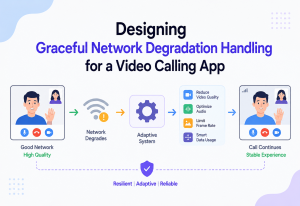
17.1 A Closer Look at the Professional-Networking Case
What makes the professional networking domain specifically different from, say, video or music recommendation, is the presence of a rich, structured professional graph layered on top of the usual content and behavioral signals. Knowing that two of your first-degree connections currently work at a company is an extraordinarily strong relevance signal — arguably stronger than almost any purely content-based feature — because it correlates both with genuine cultural/professional fit and with a concrete path to a warm referral, which dramatically increases the odds of actually landing an interview. Any credible architecture in this space treats the connection graph as a first-class feature source, not an afterthought bolted onto a generic recommender copied from e-commerce.
Similarly, the two-sided nature of this particular marketplace deserves a second look. In a movie recommender, the “supply side” (the catalog of movies) is relatively static and has no feelings about who watches it. In a job marketplace, the supply side is made up of employers who are themselves optimizing for something — a fast, high-quality pipeline of applicants — and who will simply stop posting if the platform sends them a flood of poorly-matched candidates. This means the ranking objective can never be a pure function of job-seeker delight; it must also be evaluated against downstream employer-side signals such as interview conversion rate and hire rate, closing the loop between “the user liked this recommendation” and “this recommendation actually worked for both sides of the marketplace.”
- “Can you name a company using a similar two-stage retrieval-then-ranking pattern outside of job platforms, and explain why the pattern transfers?”
- “How would you incorporate the professional connection graph as a feature, and how would you keep that computation fast at serving time?”
- “How would you factor employer satisfaction into a ranking objective that’s mostly built around job-seeker engagement?”
Frequently Asked Questions
Because scoring tens of millions of jobs per request, per user, for hundreds of millions of users, simply cannot finish inside a latency budget of a few hundred milliseconds. The two-stage design exists specifically to make the problem computationally tractable.
Cold start is handled by leaning on whatever signal does exist — even a partially filled profile (current title, location) feeds content-based filtering — combined with popularity-based fallback recommendations (trending jobs in their stated field/location) until enough personal behavioral data accumulates.
The user might briefly see a closed posting until the cache TTL expires or they click it (at which point the click handler validates the posting is still open before proceeding to the application flow) — an accepted, deliberate trade-off between freshness and system load.
Search is pull-based and query-driven (the user tells you what they want via keywords); recommendation is push-based and profile/behavior-driven (the system infers what they want without an explicit query). Most platforms run both, sharing infrastructure like the job index, but with very different ranking logic.
A combination of offline metrics (recall@K, NDCG against historical logs) before ever showing users anything, followed by online A/B testing measuring click-through rate, application rate, and longer-term retention/hire outcomes once live.
Embeddings capture semantic similarity — “Software Engineer” and “Backend Developer” land close together in vector space even though they share no exact keywords, letting the system catch relevant jobs that keyword matching alone would completely miss.
There’s no universal answer, but a common pattern is a full retrain on a regular cadence (daily or weekly) combined with continuous monitoring for prediction drift, triggering an earlier retrain if the live data distribution shifts noticeably away from what the model was trained on — for example, after a sudden change in the job market.
Cold start refers to the difficulty of making good recommendations when there isn’t yet enough data — either for a brand-new user (no click/apply history) or a brand-new job posting (no engagement history). It’s never fully “solved,” only mitigated: content-based signals and reasonable defaults (popularity, recency) fill the gap until enough behavioral data accumulates to hand off to the stronger collaborative and learned-ranking signals.
They typically share underlying infrastructure (the same Job Postings DB, the same Search Index, often the same Feature Store) but use different ranking logic — search ranking weighs query-term match heavily, while the recommendation feed ranking weighs profile and behavioral similarity heavily, with little to no explicit query at all.
First, offline evaluation against historical logs using metrics like recall@K and NDCG (Normalized Discounted Cumulative Gain) to see if it would have ranked known-good outcomes higher. Then, shadow traffic — running the new model alongside the current production model on live traffic without actually showing its results to users, comparing their outputs. Only after both pass do you move to a small canary rollout to real users.
Summary & Key Takeaways
We started with a single sentence — “show me the jobs that matter to me, out of millions” — and built it into a full, production-grade architecture: an edge layer (Load Balancer, API Gateway), a two-stage recommendation core (Candidate Generation over a Vector Database, then a Ranking Service backed by a Feature Store), a real-time activity pipeline (Kafka + stream processing), an offline training loop feeding a Model Registry, and reliability, security, and observability wrapped around every layer.
If there is one habit worth carrying forward from this entire exercise, it’s this: every box in Fig 1 exists because it answers a specific, previously stated problem — not because it looked impressive on a diagram. The Load Balancer exists because a single server cannot survive real traffic. The two-stage retrieval pattern exists because scoring every job for every user cannot fit inside a latency budget. The Feature Store exists because training and serving must see identical computations or the model silently misbehaves. The circuit breaker exists because a dependency will eventually fail, and the system must degrade gracefully rather than collapse entirely. Approached this way — always tracing a component back to the concrete problem it solves — system design stops being a memorization exercise and becomes something closer to engineering judgment, which is exactly the skill this kind of system, and this kind of interview question, is actually testing.
Key Takeaways
- Two-stage retrieval is the core enabling pattern — cheap recall, then precise ranking on a small shortlist.
- Freshness matters as much as relevance — a perfectly matched but closed job is useless.
- Cold start needs explicit design — content-based fallback for new users and new jobs alike.
- A feature store prevents train/serve skew — arguably the most common silent ML bug in production.
- Graceful degradation beats perfect availability — a cached or simplified feed is always better than none.
- Privacy is uniquely high-stakes in this domain — leaking job-search activity can cost someone their livelihood.
- Optimize a blended objective, not raw CTR alone, to avoid rewarding clickbait-y postings.
- Everything is independently scalable — stateless services, sharded data stores, and batched ML inference.
- Canary rollouts protect against model regressions before they hit 100% of users.
- Little’s Law gives a concrete, defensible way to size a service’s concurrency needs from arrival rate and processing time.
Great recommendation systems are not built by chasing a single clever model — they are built by ensuring that every component of the pipeline, from candidate generation to ranking to caching to graceful degradation, was chosen deliberately to answer a specific, well-stated problem. Do that consistently, at every layer, and both the system and the interview answer around it stop feeling like magic and start feeling like engineering.