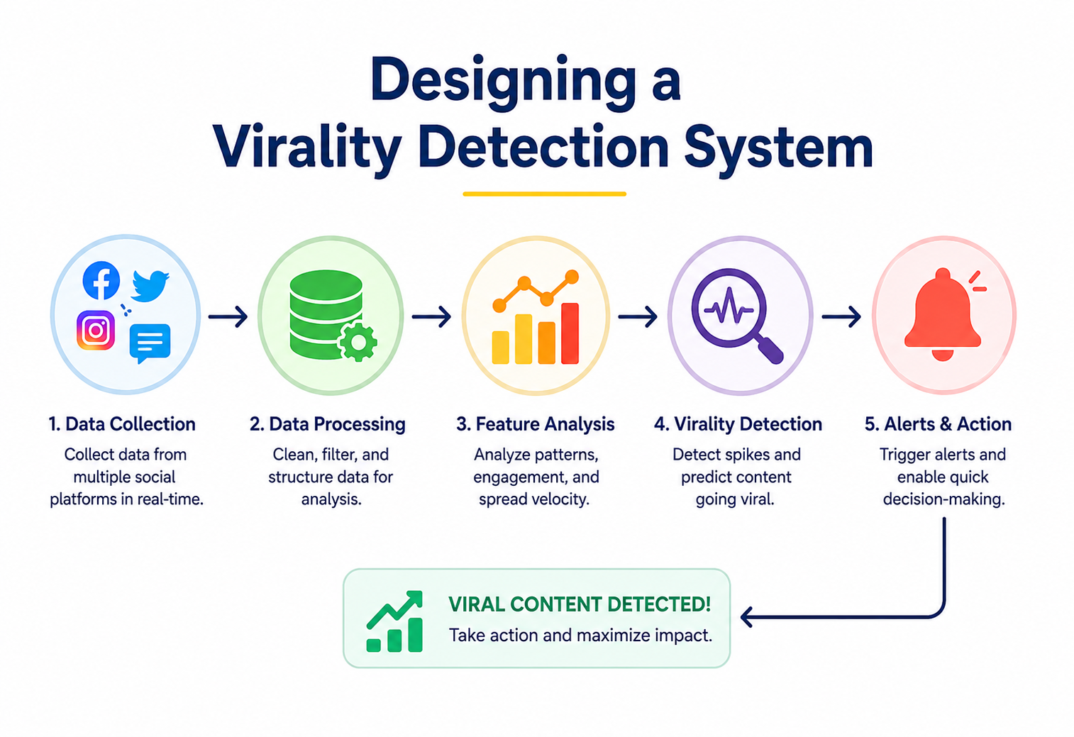
Designing a system that spots viral content before the crowd does
A complete, ground-up walkthrough of how to build a platform that watches engagement signals as they happen and flags posts that are about to explode — minutes or hours before a human would ever notice.
Why This Problem Matters
Every platform that hosts user-generated content — a video app, a social feed, a marketplace of reviews, a forum — has a small, invisible team working around the clock: content moderators, growth marketers, editors and recommendation algorithms, all trying to answer one question. Which piece of content is about to matter a lot more tomorrow than it does right now?
For most of the internet’s history, this question was answered after the fact. A post would get shared thousands of times, a moderator would eventually notice a wave of reports, a marketing team would spot a trending hashtag hours after it started trending. By the time anyone reacted, the moment had already happened. The platform was a spectator to its own content, not a participant.
Virality prediction flips that timeline. Instead of asking “what went viral yesterday”, a virality detection system asks, continuously and automatically, “what is about to go viral in the next few hours” — while there is still time to act on the answer. That single shift, from looking backward to looking forward, is what makes this one of the more interesting real-time systems to design, because it forces you to solve streaming data, machine learning and distributed systems problems all at once, under a strict time budget.
Think about how a seismologist works. They do not wait for an earthquake to happen and then report it — that is just news. Their real job is reading tiny, continuous tremors from sensors buried across a region and asking whether those tremors are the early signature of something much bigger. A single tremor means nothing. A rising pattern of small tremors, all pointing the same direction, is the signal worth an alarm. A virality detection system does exactly this, except the “tremors” are likes, shares, comments and watch-time and the “sensors” are your application servers.
This dynamic also explains why the problem resists simple solutions borrowed from adjacent domains. Fraud detection, for comparison, usually has the luxury of a slightly longer decision window and a well-understood set of known attack patterns to check against. Virality detection has neither luxury: the decision window is measured in minutes and the underlying phenomenon being detected — genuine, organic, human enthusiasm compounding on itself — has no fixed signature to pattern-match against, only a statistical shape that has to be learned and continuously re-learned as content, audiences and platforms themselves keep changing.
Who actually needs this
Social & video platforms
Decide what to push into recommendation feeds before the crowd finds it organically, so early promotion compounds the effect.
Trust & safety teams
Get ahead of harmful or misleading content that is about to reach a mass audience, instead of reacting to it after millions of views.
Marketing & PR
Brands and agencies want early warning that a piece of content mentioning them is heating up, good or bad, while there is still time to respond.
Infrastructure teams
Viral content causes traffic spikes on specific URLs, CDNs and databases. Predicting it ahead of time lets you pre-scale, not just autoscale reactively.
Why “before it happens” is the whole point
It is worth pausing on why the timing constraint is so central to this entire design, rather than a nice-to-have. A system that identifies viral content accurately but only after it has already peaked provides essentially no actionable value — the recommendation system has nothing left to boost, the trust and safety team has nothing left to prevent and the marketing team has nothing left to plan around. Every architectural decision that follows in this guide, from choosing a streaming pipeline over a batch job, to accepting a noisier cold-start heuristic over waiting for a fully confident prediction, to building graceful degradation instead of simply going offline under load, ultimately traces back to protecting that early-warning window. Losing accuracy at the margins is often an acceptable trade; losing the lead time is not, because lead time is the entire reason the system exists in the first place.
The core difficulty
The hard part is not building a dashboard that shows what is currently popular — that is a simple counting problem. The hard part is separating a post that is genuinely accelerating from one that merely got a normal early burst and will plateau. Most content that gets 100 likes in the first ten minutes never becomes viral. A small number of posts that also get roughly 100 likes in the first ten minutes go on to reach millions. From the outside, in that first window, they can look nearly identical. The system has to learn the subtle difference in the shape of engagement, not just its size.
“Why cannot you just alert when a post crosses a fixed threshold, like 1,000 likes per minute?” A strong answer explains that fixed thresholds fail across content types, audience sizes and time zones — a post from an account with 50 million followers reaches 1,000 likes/minute trivially and routinely, while the same rate from a brand-new account is extraordinary. The system needs relative, learned signals, not one global constant.
A brief history of the problem
Early social platforms handled “what is popular” with the simplest tool available: a leaderboard, sorted by raw counts, refreshed on some batch schedule — hourly or even daily. This was cheap to build and good enough when content volume was low and human editors could still plausibly review everything by hand. As platforms scaled into the millions and then billions of daily posts, two things broke at once: batch refresh cycles became far too slow to be useful for anything time-sensitive and the sheer volume made manual review of every candidate completely impractical. The industry’s response was a gradual shift toward streaming architectures — computing trends continuously rather than in periodic batches — followed by a second shift toward prediction rather than pure measurement, once it became clear that reacting to a trend after it was already visible to users was, in a competitive sense, already too late. The system described in this guide sits at the current end of that evolution: a fully streaming, predictive approach, built on the same underlying stream-processing technology that also modernised fraud detection, ad auction pricing and real-time personalisation across the industry over roughly the same period.
What makes this different from a generic anomaly detector
It is tempting to treat this as “just” an anomaly detection problem — find the data point that deviates from the norm. That framing is useful but incomplete. A generic anomaly detector is agnostic about direction and cause; it flags anything unusual, whether that is a sudden crash in engagement, a data pipeline bug producing garbage numbers, or genuine organic growth. A virality detection system needs to be far more specific: it must distinguish a genuinely compounding, self-sustaining growth pattern from a one-time burst that will not continue, using domain-specific structure (the K-factor concept from Section 2) rather than generic statistical deviation alone. That distinction — compounding growth versus a one-time burst — is really the intellectual core of the entire system and it is why feature engineering (Section 5) carries so much of the weight relative to the choice of model algorithm.
Core Concepts & Vocabulary
Before touching architecture, it helps to build a shared vocabulary. Every term below will reappear repeatedly through the rest of this guide.
Engagement event
Any single, timestamped user action tied to a piece of content: a like, a share, a comment, a save, a click, a completed video view, a report. Each event is small, but at scale a popular platform produces hundreds of thousands of these every second.
If you post a photo and three friends like it in the first minute, that is three engagement events: (post_id, user_id, LIKE, timestamp) repeated three times.
Engagement velocity
The rate at which engagement events accumulate — typically events per minute. This is the first derivative of raw engagement count over time, the same way speed is the first derivative of distance.
Engagement acceleration
The rate at which velocity itself is changing — the second derivative. A post whose velocity is climbing (positive acceleration) is behaving very differently from one whose velocity is flat or falling, even if their current velocities happen to match at this instant. Acceleration is often the single most predictive raw signal in virality detection, because it captures momentum before absolute numbers look impressive.
Virality coefficient (K-factor)
Borrowed from epidemiology and viral marketing: on average, how many new viewers does each existing viewer bring in? If K > 1, each viewer more than replaces themselves — the audience compounds, which is the mathematical definition of “going viral”. If K < 1, the spread naturally dies out no matter how large the initial audience was.
K-factor is the same math behind how a contagious illness spreads versus a mild cold that a family catches and it goes no further. One infected person who infects 2.5 others on average produces an outbreak; one who infects 0.6 others on average produces a handful of cases that fizzle out. Content works the same way — a K-factor above 1 means the crowd is doing your distribution work for you.
Cold-start window
The earliest minutes of a post’s life, before enough data exists to be confident about its trajectory. Every prediction system has to decide how much to trust thin, noisy early signals versus waiting for more data (and losing the “before it happens” advantage in the process).
Decay-adjusted signal
Raw engagement counts favour old content — a two-year-old post naturally has more total likes than a five-minute-old one. Decay-adjusted signals apply time-weighting (often exponential decay) so recent activity counts more than stale activity, which is what lets a five-minute-old post be compared fairly against a two-year-old one.
False positive / false negative, in this context
| Term | Meaning here | Cost |
|---|---|---|
| False positive | System flags a post as “going viral” and it never does | Wasted promotion slots, wasted moderator attention |
| False negative | A post genuinely goes viral but the system never flags it | Missed growth opportunity, or missed harmful content, depending on use case |
Which error matters more is a business decision, not a technical one — a trust & safety use case usually tolerates more false positives to avoid missing harmful viral content, while a growth / recommendation use case usually tolerates more false negatives to avoid wasting limited promotional slots on posts that fizzle.
Time-to-peak
How long it takes a post to reach its maximum engagement velocity after being published. This varies enormously by content type and platform — a short clip might peak within hours, while a long-form piece might build steadily over days. Time-to-peak is useful less as a feature fed directly into the model and more as a framing tool for deciding how long the system should keep actively scoring a given post before considering it settled and moving it to the slower monitoring cadence described later in this guide.
Saturation
The point at which a post’s growth naturally slows, not because interest has died, but because it has already reached most of the audience realistically capable of seeing it — the denominator, not the numerator, has become the limiting factor. Distinguishing genuine saturation from an early plateau that might still resume accelerating is one of the more subtle judgment calls the model has to make and it is part of why acceleration, not just velocity, is such a heavily weighted feature throughout this system.
“How would you define the label for your training data — what counts as ‘went viral’?” This is a genuinely open-ended system design question. A solid answer proposes something measurable and specific, such as “reached the 99th percentile of engagement-per-hour for its content category within 24 hours of posting” and acknowledges that the threshold is a tunable business parameter, not a fixed law.
High-Level Architecture
At the highest level, this system is a real-time pipeline with five jobs: collect engagement events as they happen, turn raw events into meaningful features, score those features against a trained model, decide what to do with high-scoring posts and store enough history to keep improving the model over time. Everything below is a variation on that five-step spine.
Reading this diagram left to right tells the whole story of the system. Events enter through a lightweight gateway, land on a durable stream bus, get aggregated into time-windowed features, are scored by a model in near real time and — if the score crosses a threshold — trigger one of several downstream actions. The bottom loop is just as important as the top row: everything the system observes is also written to cold storage so that the model can be retrained on real outcomes, closing the loop between prediction and ground truth.

The five core services
| Service | Responsibility | Typical tech |
|---|---|---|
| Event Gateway | Accepts engagement events from clients, validates and enriches them, publishes to the stream bus | REST / gRPC service behind a load balancer |
| Stream Processor | Consumes the raw event stream, computes windowed aggregates (velocity, acceleration, unique reach) | Kafka Streams, Apache Flink |
| Feature Store | Serves low-latency features to the scoring service; also stores historical features for training | Redis (hot) + a columnar store (offline) |
| Scoring Service | Runs the trained model against current features and returns a virality probability | Model server, e.g. TensorFlow Serving or a custom Java service |
| Decision Service | Applies business rules to scores — thresholds, cooldowns, category-specific logic — and routes to downstream consumers | Stateless microservice |
Why a dedicated stream processor instead of computing features inside the scoring service
An early, tempting simplification is to skip the dedicated Stream Processor entirely and have the Scoring Service compute features directly from raw events on demand. This looks simpler on a whiteboard, but it breaks down under real load for a specific reason: feature computation (windowed aggregation across potentially millions of events for a single very popular post) is a fundamentally different workload from model inference, with different scaling characteristics, different failure modes and different optimal hardware profiles. Coupling them means the Scoring Service can never scale, deploy, or fail independently of feature computation and a spike in raw event volume for one extremely popular post would directly degrade inference latency for every other post being scored at the same time. Keeping them as separate services, connected only through the Feature Store, is what allows each to be reasoned about, scaled and operated independently — a recurring theme that shows up again in Section 9’s discussion of service boundaries.
The role of the offline training pipeline in the bigger picture
The bottom loop in Figure 1 is easy to treat as an afterthought next to the real-time path, but it is what keeps the entire system from becoming stale. Every prediction the system makes eventually resolves into a known outcome — the post either did or did not reach the virality threshold within the defined window — and that resolved outcome becomes a labeled training example the next time the offline pipeline runs. Without this loop, the model would be frozen at whatever it learned from its initial training set, while the platform’s content mix, audience behaviour and even adversarial manipulation tactics keep evolving underneath it. The real-time path and the offline training loop are, in a real sense, two halves of one system: one half acts on what is currently known, the other half continuously improves what is known in the first place.
“Why split the Scoring Service and the Decision Service instead of having the model directly trigger actions?” The good answer: separating “how likely is this to go viral” (a stable, reusable number) from “what do we do about it” (business logic that changes constantly, differs by team and should not require retraining a model) is a classic single-responsibility separation. It also lets multiple different downstream consumers reuse the same score with different thresholds.
Ingestion & Signal Collection
Everything the system knows starts as a raw engagement event generated somewhere on a user’s device. Getting this stage right matters more than it looks, because every downstream component inherits whatever quality problems exist here.
What actually gets captured
- Direct engagement: likes, shares, comments, saves, reactions
- Passive engagement: watch time, scroll-past rate, dwell time, replay count
- Distribution signals: how many distinct feeds or surfaces the content is currently appearing on
- Network signals: is the sharing coming from a tight, insular cluster of accounts, or spreading across otherwise-unconnected communities (a strong early indicator of genuine virality versus a coordinated but small campaign)
Short-video platforms weight watch-time and replay behaviour heavily in this stage, because a share can be gamed relatively easily, but genuinely re-watching a fifteen-second clip three times is a much harder signal to fake and correlates strongly with organic virality.
Client-side batching
Sending a network request for every single tap would overwhelm both the client’s battery and the server’s connection pool. Real systems batch events client-side and flush every one to two seconds, or immediately for a small allow-list of high-value events. This introduces a deliberate, small latency cost in exchange for a large reduction in request volume — a trade-off worth naming explicitly in a design discussion.
The event gateway
A thin, horizontally scaled service sits between clients and the stream bus. Its job is intentionally narrow: authenticate the request, validate the event shape, attach server-side metadata (a trusted timestamp, since client clocks cannot be trusted) and publish to the correct stream partition. It should do essentially no business logic — that keeps it fast and easy to scale.
public class EngagementEvent {
    private final String postId;
    private final String userId;
    private final EngagementType type;   // LIKE, SHARE, COMMENT, VIEW...
    private final long clientTimestamp;
    private final long serverTimestamp;  // authoritative, set at the gateway
    private final String surface;        // "feed", "search", "profile"...

    // constructor, getters omitted for brevity
}

public class EventGatewayController {

    private final KafkaProducer<String, EngagementEvent> producer;

    public Response ingest(RawEventPayload payload) {
        if (!Validator.isWellFormed(payload)) {
            return Response.badRequest("malformed event");
        }

        EngagementEvent event = EngagementEvent.builder()
            .postId(payload.getPostId())
            .userId(payload.getUserId())
            .type(payload.getType())
            .clientTimestamp(payload.getClientTimestamp())
            .serverTimestamp(System.currentTimeMillis())  // never trust the client
            .surface(payload.getSurface())
            .build();

        // partition key = postId, so all events for one post land on the same partition
        // this keeps ordering guarantees intact for the stream processor
        producer.send(new ProducerRecord<>("engagement-events", event.getPostId(), event));

        return Response.accepted();
    }
}
Notice the partition key choice: every event for a given post is routed to the same Kafka partition. This single decision is what allows the stream processor downstream to compute per-post windowed aggregates without needing to coordinate across machines — a good example of how an early design choice quietly simplifies a much bigger component later.
Schema evolution
An engagement event schema is never truly final — new engagement types get added as the product evolves (a “save to collection” feature launching two years after the platform itself) and older event producers on outdated app versions will keep sending the old schema for a long time after a new one ships. The event gateway and the stream processor both need to tolerate this gracefully: a schema registry that enforces backward and forward compatibility rules (new fields are optional with sensible defaults, existing fields are never repurposed or removed outright) keeps the pipeline from breaking every time the event shape changes and keeps years-old mobile app versions from silently corrupting the stream.
Ordering guarantees and why they matter here specifically
Because the stream processor computes running windowed aggregates incrementally (Section 16b covers the sliding-window technique), it implicitly assumes it sees a post’s own events in roughly the order they occurred. Out-of-order delivery does happen in practice — a mobile client batching and flushing events on a delay, as described above, plus normal network jitter — so the stream processor needs an explicit strategy for late or out-of-order events: a small allowed lateness window (commonly a few seconds to a couple of minutes) during which a late-arriving event can still be folded into the correct time window, with anything later than that either dropped or corrected in a small side-channel adjustment rather than reopening and recomputing a window that has already been used to make live decisions.
“What happens if the event gateway is briefly unavailable?” The expected answer covers client-side retry with exponential backoff and local buffering, so a two-second network blip does not silently drop engagement data — which would be especially bad given that this data is the entire input to the model.
Feature Engineering
Raw events are not useful to a model on their own — a model cannot learn from a firehose of individual likes. The stream processor’s job is to turn that firehose into a small number of dense, meaningful numbers, refreshed continuously, for every active post. This is where most of the actual “intelligence” of the system lives, arguably more than in the model itself.
Windowed aggregation
The stream processor maintains rolling windows per post — commonly 1-minute, 5-minute, 30-minute and 3-hour windows, each sliding forward continuously. For every window, it computes counts per engagement type, unique-user counts (to detect a small number of accounts inflating numbers) and velocity relative to the previous window.
Key engineered features
| Feature | Why it matters |
|---|---|
| velocity_5m / velocity_30m ratio | Captures whether momentum is accelerating (ratio > 1) or fading (ratio < 1), independent of raw scale |
| unique_user_ratio | Distinct engagers ÷ total engagements. A low ratio can flag bot activity or a small coordinated group rather than organic spread |
| audience_diversity | How spread out the engaging accounts are across social clusters — organic virality tends to jump between clusters; a manufactured spike tends to stay within one |
| comment_sentiment_velocity | Rate of change of sentiment in early comments; strong reactions (positive or negative) often precede virality more than neutral ones |
| creator_baseline_deviation | How far this post’s early performance deviates from that specific creator’s historical average — critical for fairness across account sizes |
| time_since_post | Same absolute velocity means something very different at minute 3 versus minute 90 |
Creator baseline deviation is like a doctor reading vital signs. A resting heart rate of 100 is unremarkable for someone who just finished sprinting and alarming for someone lying still. The absolute number means nothing without a personal baseline to compare it against — which is exactly why the system tracks each creator’s own historical patterns rather than one global number.
Feature freshness trade-off
Longer windows (3 hours) are more statistically stable but slower to reflect brand-new momentum. Shorter windows (1 minute) react instantly but are noisy — a single influencer share can distort a 1-minute window dramatically. Production systems combine both: short windows detect the earliest hint of movement, longer windows confirm the pattern is real rather than a blip.
Normalisation across content categories
A raw feature like velocity_5m means something completely different for a short-form video than for a long-form written post, simply because the two content types have entirely different baseline engagement rates and entirely different typical time-to-peak. Feeding raw, un-normalised values from every content category into one shared model forces it to implicitly relearn these differences from data, which wastes model capacity and makes the model more fragile whenever the platform introduces a genuinely new content format. A cleaner approach normalises each feature relative to a rolling baseline computed separately per content category — expressing velocity as a z-score relative to that category’s recent distribution rather than as a raw count — so the model itself can stay simpler and more directly comparable across very different kinds of content.
Feature staleness handling
A feature vector is only as good as how current it is and different features go stale at different rates. Engagement velocity needs to be nearly real time to be useful at all, since its entire value lies in reflecting what is happening right now. Creator baseline statistics, by contrast, change slowly and can be refreshed on a much longer cycle — hourly or daily — without meaningfully affecting prediction quality. Treating every feature as needing the same refresh cadence wastes compute on the slow-changing ones and, worse, can create unnecessary load on the pipeline precisely during the high-traffic moments when that capacity is needed most for the features that actually matter in the moment.
“How do you handle a feature store that needs to serve both low-latency reads for scoring and large historical reads for training?” A well-prepared answer proposes a hot/cold split: a low-latency store like Redis holding only the current feature vector for active posts, alongside an offline columnar store (or data lake table) holding the full feature history for model training — the classic Lambda-style split between a speed layer and a batch layer.
The Prediction Engine
With a clean feature vector per post, refreshed every few seconds, the system needs a model that converts that vector into a single virality probability. This section covers what kind of model fits the problem and how it is served at low latency.
Framing the ML problem
This is best framed as a binary classification problem with a time-decaying label: given a post’s feature vector at time t, will it reach the top percentile of engagement for its category within the next 24 hours? Framing it as classification (rather than regression on raw future engagement count) is deliberate — the business action (“promote it” or “flag it”) is itself binary and classification models tend to be more robust to the extreme skew in engagement counts, where a handful of posts get orders of magnitude more engagement than everything else.
Model choice
Gradient-boosted trees (such as XGBoost or LightGBM) are a strong default here, for a specific reason: the engineered features above are tabular, heterogeneous in scale and full of interaction effects (velocity matters differently depending on time_since_post) — exactly the conditions where tree ensembles outperform deep learning without needing anywhere near as much training data or infrastructure. Deep learning becomes worth the added complexity mainly when raw content (text, image or video embeddings) is folded in directly, rather than only hand-engineered numeric features.
It is worth being explicit about the counterargument too, since a good system design discussion should acknowledge trade-offs rather than presenting one option as obviously correct. A deep model, particularly one that ingests raw content embeddings alongside behavioural features, can in principle capture patterns that hand-engineered features miss entirely — a specific visual style, a particular narrative structure, or subtle linguistic patterns that correlate with virality in ways no one thought to encode explicitly as a feature. The trade-off is real: substantially higher training data requirements, materially higher serving cost and latency and a meaningfully harder explainability story. Most teams building this kind of system start with the tree-based approach precisely because it reaches a strong baseline quickly and cheaply and only invest in a deep model once the tree-based baseline’s error patterns clearly point to missing content-level signal that no amount of additional behavioural feature engineering can recover.
A common, effective pattern combines a gradient-boosted tree model on engagement-shape features with a separate, pre-computed content-embedding similarity score — how similar this post’s content is, semantically, to other posts that have historically gone viral — fed in as just one more feature. This gets most of the benefit of deep content understanding without needing a full end-to-end deep model in the hot path.
Serving the model in real time
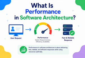
Inference has to happen inside a strict latency budget — typically under 50 milliseconds — because it runs continuously for every active post, not once per user request. A dedicated model-serving layer (TensorFlow Serving, Triton, or an embedded model inside a lightweight Java or Python service) loads the current model version into memory and exposes a scoring endpoint that the stream pipeline calls on every feature refresh.
public class ScoringService {

    private final ViralityModel model;  // loaded once, kept hot in memory
    private final FeatureStoreClient featureStore;

    public ViralityScore score(String postId) {
        FeatureVector features = featureStore.getLatest(postId);

        if (features.isColdStart()) {
            // too little data yet - fall back to a simpler heuristic model
            // rather than a noisy prediction from the full model
            return coldStartHeuristic(features);
        }

        double probability = model.predict(features);
        double confidence  = model.predictionConfidence(features);

        return new ViralityScore(postId, probability, confidence, System.currentTimeMillis());
    }

    private ViralityScore coldStartHeuristic(FeatureVector f) {
        // simple rule: is early velocity already an outlier for this content category?
        double zScore = (f.velocity5m() - f.categoryMeanVelocity()) / f.categoryStdDevVelocity();
        double approxProb = Math.min(1.0, Math.max(0.0, zScore / 5.0));
        return new ViralityScore(f.postId(), approxProb, "LOW", System.currentTimeMillis());
    }
}
The cold-start fallback matters more than it might look at first glance. In the first few minutes of a post’s life, the full model simply has not seen enough signal to be reliable and a confident-looking wrong prediction is worse than an honest, low-confidence heuristic. This is a recurring theme in real-time ML systems: knowing when not to trust the sophisticated model is as important as the model itself.
Explainability as a design requirement, not an add-on
Because this system’s predictions directly drive consequential actions — promoting a post, or routing it to a trust & safety queue — the model’s output cannot be a pure black box if the organisation wants people to trust and act on it confidently. Tree-based models have a genuine practical advantage here: techniques like SHAP (SHapley Additive exPlanations) values can attribute a specific prediction back to individual feature contributions, so a reviewer can see, for a specific post, that the flag was driven primarily by acceleration and audience diversity rather than by raw follower count, for instance. This is part of why the feature snapshot is included directly in the API response shown in Section 9 — explainability was treated as a first-class requirement of the response contract, not something bolted on later through a separate debugging tool.
Ensembling and calibration
A single gradient-boosted tree model is a strong baseline, but production systems commonly combine it with a second, simpler model trained specifically to catch a different failure mode — for example, a lightweight model focused purely on very early cold-start signals, blended with the primary model as more data becomes available, rather than switching abruptly between the two. Equally important and often overlooked, is calibration: a raw model score of 0.8 should genuinely correspond to roughly an 80% chance of the outcome occurring, not just a relative ranking. Calibration techniques (such as fitting a simple logistic or isotonic regression on top of the raw model output) matter a great deal here specifically because downstream consumers, like the Decision Service, apply fixed probability thresholds — an uncalibrated model can silently distort exactly how those thresholds behave in practice, even if its relative ranking of posts is perfectly fine.
Model retraining loop
“How would you evaluate whether a new model version is actually better before fully replacing the old one?” The strong answer is shadow deployment: run the new model on live traffic in parallel, log its predictions without acting on them and compare against real outcomes and the incumbent model over a defined period, before switching traffic over — never trust offline metrics alone for a system this sensitive to distribution shift.
Data Flow & Lifecycle
It helps to trace one single post through the entire system, start to finish, to see how every component from the last three sections connects in practice.
Why a cooldown timer matters
Without a cooldown, a post hovering right at the decision threshold could trigger the same downstream action dozens of times per minute as its score flickers above and below the line — flooding the recommendation system or a moderation queue with duplicate signals. A simple cooldown (for example, “do not re-fire for this post for at least 10 minutes after a decision”) keeps the system stable without needing a more complex debouncing mechanism.
End-of-life for a post’s hot data
Not every post stays “active” in the hot feature store forever — that would grow unbounded. Once a post’s velocity has stayed below a low threshold for a defined period (say, one hour), its hot feature entry is evicted from the low-latency store and the post is considered dormant. If engagement later reactivates (a post resurfacing after a celebrity mention, for instance), a new event simply re-triggers hot-path processing for it — the design should assume dormancy is temporary, not permanent.
Storage, Caching & Queues
Why Kafka (or an equivalent log) sits at the centre
A distributed commit log is the right backbone here for three reasons: it decouples producers (the event gateway) from consumers (the stream processor, the archival job, any future consumer) so new downstream services can be added without touching ingestion; it provides ordering guarantees per partition, which the windowed aggregation logic depends on; and it provides durability and replay — if the stream processor crashes, it resumes from its last committed offset rather than losing data.
A commit log is like a conveyor belt with a permanent, ordered record of everything that has passed by, rather than a hallway where messages get handed directly from one person to another. Anyone can walk up to the belt and start reading from wherever they left off, even hours later, without disturbing anyone else reading the same belt.
Storage tiers
| Tier | Technology | What lives here | Latency |
|---|---|---|---|
| Hot cache | Redis / in-memory KV store | Current feature vector per active post | < 5 ms |
| Operational DB | Wide-column store (e.g. Cassandra / Bigtable-style) | Recent event history per post, decision logs | ~10-30 ms |
| Cold storage / data lake | Object storage + columnar tables (Parquet) | Full historical events, features and outcomes for training | seconds-minutes (batch) |
Why not just use the primary database for everything
The read/write pattern here is fundamentally different from a typical CRUD application: extremely high write throughput (every engagement event), extremely frequent small reads for scoring (every few seconds per active post) and only occasional large batch reads for training. A single general-purpose relational database struggles to serve all three patterns well simultaneously — which is exactly why this architecture splits storage by access pattern rather than trying to force one system to do everything.
Caching the feature vector, not just the raw counts
It is tempting to cache raw engagement counters and recompute derived features (velocity, acceleration) on every read. In practice, precomputing the full feature vector in the stream processor and caching the finished vector is far cheaper, because the scoring service can then be a very simple, very fast reader with no computation of its own — pushing complexity upstream to where it only has to happen once per update, not once per read.
Replication and partitioning of the operational store
The wide-column operational database sitting between the hot cache and cold storage typically partitions data by post ID, the same key used throughout the pipeline, so that all the recent event history for a given post lives together and can be retrieved with a single targeted read rather than a scatter-gather query across many nodes. Each partition is replicated across multiple nodes (commonly three, a widely used default that tolerates a single node failure while still allowing a majority quorum for writes), so a single node failure does not cause data loss or even a visible availability gap for reads and writes to posts on that partition. This partition-plus-replica structure is a standard pattern across most horizontally scaled data stores and it is worth being able to describe it generically in an interview setting, independent of any single specific database product.
Time-to-live and data lifecycle
Not all data in this pipeline needs to live forever and being deliberate about lifecycle policy is both a cost control and a genuine architectural decision. Hot cache entries expire on the order of hours, tied to the dormancy logic from Section 7. Operational store entries — recent event history — might be retained for a few weeks, long enough to support debugging a recent incident or reprocessing a recent time range if a bug is found in the feature computation logic. Cold storage retains data far longer, often a year or more, because the training pipeline benefits from seeing how engagement patterns shift across seasons and platform growth phases and because certain trust-and-safety or compliance requirements may mandate longer retention regardless of what the model itself needs.
“Your Redis feature cache goes down. What happens to the system?” The expected discussion: scoring should degrade gracefully rather than fail outright — falling back to a slightly stale read from the operational database, or briefly widening the scoring interval, is preferable to the whole prediction pipeline going dark. This is a good moment to bring up circuit breakers and graceful degradation explicitly.
APIs & Microservices
The system is naturally organised as a small set of independently deployable services, each owning one part of the pipeline. This section covers the contracts between them.
Why async between some services and sync between others
The links carrying continuous high-volume data (events, scores flowing to consumers) are asynchronous, so a slow or temporarily unavailable downstream service never blocks upstream processing. The link from the Feature Store to the Scoring Service is synchronous because scoring genuinely needs the freshest possible read at the moment of inference — there is no benefit to decoupling a read that must happen right now.
Sample API — Decision Service
{
  "postId":       "p_9f21ac",
  "score":        0.87,
  "confidence":   "HIGH",
  "decidedAt":    "2026-07-28T09:12:44Z",
  "action":       "PROMOTE",
  "cooldownUntil":"2026-07-28T09:22:44Z",
  "featureSnapshot": {
    "velocity5m":       412.3,
    "acceleration":     38.1,
    "uniqueUserRatio":  0.94
  }
}
Exposing a feature snapshot alongside the score is a deliberate design choice, not an afterthought — it makes the decision auditable. When a human later asks “why was this post promoted”, the answer is inspectable rather than a black box, which matters enormously for the trust & safety use case in particular.
Idempotency
Because events can be redelivered (a consumer crash-and-restart, a network retry), every stage needs to handle duplicate events safely. Engagement events carry a unique event ID; the stream processor deduplicates using a short-lived window of recently seen IDs before folding an event into its aggregates, preventing a single retried “like” from being double-counted.
API versioning across independently deployed services
Because each service in this architecture deploys independently, the contracts between them need explicit versioning rather than an implicit assumption that every service is always running the latest build. The feature vector schema, the score message format and the decision API shown above should all carry an explicit version field and consuming services should be written to tolerate unknown, additional fields gracefully rather than breaking on anything they do not recognise. This additive, tolerant-reader approach is what lets one team ship a new feature to the Stream Processor on Tuesday without coordinating a simultaneous deployment of the Scoring Service, the Decision Service and every downstream consumer on the same day — a coordination cost that would otherwise slow the whole system down considerably as more teams and consumers get added over time.
“How do you prevent the Decision Service from double-triggering a promotion if it receives the same score message twice?” Expect a discussion of idempotency keys — the Decision Service should key its actions on (postId, decisionWindow) and check-and-set against a store before acting, so a duplicate message is a safe no-op rather than a duplicate promotion.
Scalability & Performance
Where the scale pressure actually is
The hardest scaling problem in this system is not steady-state load — it is the fact that engagement is wildly non-uniform across posts. A tiny fraction of posts (the very ones the system exists to detect) can generate a disproportionate share of all events at any given moment. This is a classic hot-key problem and it shapes several design decisions already covered above.
Partitioning strategy
Partitioning the event stream by post ID (as shown earlier) is efficient for the common case, but a single post going viral can itself overwhelm a single Kafka partition. Production systems handle this with a hybrid key: hash(postId) + timeBucket, spreading a single very-hot post’s events across a small number of partitions rather than exactly one, while still keeping each partition’s data ordered enough for correct windowed aggregation with a small merge step at read time.
Horizontal scaling per component
| Component | Scales by | Notes |
|---|---|---|
| Event Gateway | Stateless replicas behind a load balancer | Trivial to scale; no shared state |
| Stream Processor | Consumer group parallelism, one instance per partition | Scale by increasing partition count ahead of demand |
| Feature Store (hot) | Sharded Redis cluster | Shard by postId; watch for hot shards during real viral events |
| Scoring Service | Stateless replicas, model held in memory | CPU-bound; scale on inference latency, not just request count |
Backpressure
When the stream processor falls behind consumption (say, during an actual viral event, ironically the exact moment accuracy matters most), the system needs a defined degradation strategy rather than an unbounded queue backing up. A common approach: widen the aggregation window’s refresh interval under load — score every 15 seconds instead of every 3 — trading a small amount of detection latency for system stability, rather than falling over entirely.
Large-scale feed platforms apply adaptive sampling under extreme load: once a post’s velocity is already unambiguously in “definitely going viral” territory, the system can safely process every Nth event rather than every single one for that post, since the statistical signal barely changes while the processing cost drops substantially — a pragmatic trade only worth making at the very top of the distribution.
Capacity planning and load testing
Because the load pattern is so uneven, capacity planning based on average traffic is close to useless for this system; what matters is planning around the shape of realistic worst-case bursts. A common practice is to replay historical event logs from a genuine past viral event at increasing speed multipliers against a staging environment — two times real speed, five times, ten times — to find the point at which each component’s latency starts degrading and to make sure that point sits comfortably above any burst the system has actually seen historically, with margin for future growth in the platform’s overall user base. This kind of replay-based load testing tends to surface far more realistic bottlenecks than synthetic uniform-load testing, precisely because it preserves the bursty, single-post-dominated shape that synthetic load generators often smooth away by spreading load evenly across many keys.
Autoscaling lag and pre-warming
Reactive autoscaling — adding capacity once utilisation crosses a threshold — has an inherent lag of anywhere from tens of seconds to a few minutes, which is often exactly the window where an early, still-forming viral event needs the most headroom. Some platforms mitigate this with lightweight predictive pre-warming: using coarse, cheap early signals (for instance, unusually rapid growth in an account’s follower count, or a sudden surge of external referral traffic pointing at the platform) as a trigger to proactively scale up affected components slightly ahead of the engagement event traffic itself arriving, rather than waiting for the engagement traffic to cross a utilisation threshold after the fact.
“Walk me through what happens end to end when a celebrity posts something and engagement events spike 200x in sixty seconds.” A complete answer touches partition-level hot-keying, autoscaling lag (new consumer instances take time to spin up), backpressure / adaptive sampling as a stopgap and the fact that the cold-start heuristic model may briefly be more useful than the full model if features are refreshing faster than the model can be re-scored meaningfully.
Reliability & High Availability
What “available” means for this system
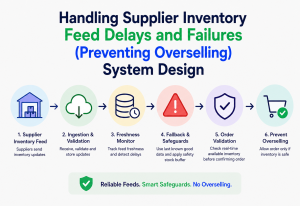
A brief outage in the Scoring Service does not lose data — events keep flowing into Kafka and features keep updating, so predictions simply resume once the service recovers, with no permanent loss. This is a genuinely useful property to design toward deliberately: separate the durable, replayable parts of the pipeline (anything backed by the commit log) from the ephemeral, in-memory parts (the current model’s hot state) and accept that only the latter needs true zero-downtime guarantees.
Graceful degradation ladder
- Full health: full model, freshest features, sub-second decision latency.
- Feature store degraded: fall back to slightly stale reads from the operational database; log a warning, keep serving.
- Scoring service degraded: fall back to the cold-start heuristic for all posts, not just new ones — a rough signal beats no signal.
- Full pipeline outage: stop making automated promotion decisions; surface a clear “predictions unavailable” state to any dependent dashboards rather than silently returning stale or default scores as if they were current.
Defining this ladder explicitly, ahead of time, is what turns “the system is down” into “the system is operating at reduced confidence” — a much better outcome for every team depending on it.
Defining SLOs that reflect what actually matters
A generic uptime SLO — “the Scoring Service is available 99.9% of the time” — does not capture the thing users of this system actually care about, which is closer to “the system flags genuinely viral content early enough to act on it”. A more meaningful service-level objective for this domain blends availability with detection latency directly: for example, “95% of posts that reach the virality threshold are flagged within 30 minutes of crossing it and the pipeline is available to make a decision at all at least 99.9% of the time”. Framing SLOs around the actual value the system delivers, rather than around infrastructure uptime alone, tends to produce much more useful conversations during incident review than a purely technical availability number ever does on its own.
Disaster recovery
Because the commit log is the durable source of truth, disaster recovery for this system is largely a story about Kafka’s own cross-region replication and the offline data lake’s backup policy, rather than anything unique to the ML components. The model itself is trivially recoverable — it is just an artifact in a versioned registry, easy to redeploy from scratch in a new region.
“Your primary region goes down entirely. How much data, if any, is lost?” Look for an answer that separates in-flight, unreplicated events (a small, bounded window of potential loss, governed by the replication lag) from anything already committed and replicated, which survives the failover intact.
Security
Threats specific to this system
Beyond standard application security (authentication, encryption in transit and at rest, least-privilege access), a virality detection system has a threat that is unusually specific to what it does: engagement manipulation — bad actors deliberately trying to trick the model into flagging content as viral when it is not, in order to receive free promotion.
Defending against manipulation
- Bot and coordination detection: the unique_user_ratio and audience_diversity features from Section 5 exist specifically to make manufactured engagement look statistically different from organic engagement — a small, tightly connected cluster of accounts liking something rapidly has a very different signature than a genuine cross-community spread.
- Rate limiting per account: the event gateway caps how many engagement events a single account can generate per post per minute, independent of any ML-based detection, as a cheap first line of defence.
- Device and account reputation scoring: engagement from freshly created or historically low-trust accounts is down-weighted in feature computation rather than excluded outright, which avoids a hard cutoff attackers could probe around.
This is similar to how a credit card fraud system does not just block a transaction because it is large — it looks at whether the pattern of the transaction matches the cardholder’s normal behaviour. A virality system does not block engagement because it is fast — it looks at whether the shape of that engagement matches organic human behaviour.
Data access boundaries
The feature vectors and decision logs contain behavioural data about real users and creators, so access needs to be scoped tightly: the Scoring Service should only be able to read features, never raw event-level user identifiers; downstream consumers like the Trust & Safety Console need broader access than the Recommendation System and that difference should be enforced by service-level authorisation, not just convention.
Privacy considerations
Engagement events are, fundamentally, behavioural data about real people and that carries privacy obligations independent of the manipulation-detection concerns above. A few practical implications follow directly from that: the feature store should hold aggregated, derived signals rather than raw per-user engagement history wherever the model does not specifically need the latter; access to any component capable of reconstructing an individual user’s specific engagement pattern across posts should be far more restricted than access to an aggregate velocity number; and data retention policy (Section 8) should align with whatever regulatory regime applies to the platform’s user base, since indefinite retention of granular behavioural data is often the first thing a privacy review will flag. None of this is unique to virality detection specifically, but it is easy to overlook in a system whose primary framing is “engineering problem” rather than “data about people” and a thorough design discussion should name it explicitly rather than leaving it implicit.
Encryption and transport security
Every hop in the pipeline that crosses a network boundary — client to event gateway, gateway to Kafka, service to service — should run over TLS and data at rest in the operational store and cold storage should be encrypted using platform-standard mechanisms. None of this is specific to virality detection, but it is worth stating plainly in any system design discussion rather than assuming it as implicit background, since interviewers sometimes deliberately probe whether a candidate treats security as a first-class concern or only mentions it when directly prompted.

“How would someone try to game this system and how would you catch it?” Strong candidates describe a concrete manipulation strategy (e.g., a bot farm generating rapid likes) and then explain which specific feature would expose it (low unique_user_ratio, low audience_diversity, low-reputation accounts), showing they understand the feature design is not just about accuracy — it is partly a security control.
Monitoring & Observability
Metrics that matter beyond standard infra metrics
| Metric | Why it is tracked |
|---|---|
| End-to-end detection latency | Time from event ingestion to a decision being made — the core value proposition of the whole system |
| Precision @ decision time | Of posts flagged as viral, what fraction actually reached the virality threshold within 24h — measured continuously as outcomes resolve, not just at training time |
| Recall @ decision time | Of posts that did go viral, what fraction were flagged before they peaked |
| Feature staleness | Age of the feature vector used for the most recent score — a growing number signals the pipeline is falling behind |
| Model drift | Statistical distance between the current live feature distribution and the distribution the model was trained on |
The precision and recall metrics above are unusual compared to a typical service dashboard, because they can only be computed with a delay — you do not know whether a flagged post “actually” went viral until enough time has passed. This means the monitoring system itself needs a windowed, lagging evaluation job, separate from the real-time dashboards that track latency and throughput.
Tracing a single decision
Every event, feature update and score should carry a correlation ID tied to the post, so an engineer can trace a single post’s entire journey through the pipeline during an incident — from the first engagement event, through every feature refresh, to the final decision — without having to reconstruct it manually from separate logs.
Alerting philosophy: page for latency, review for quality
It is worth drawing a hard line between metrics that should wake someone up at 3 a.m. and metrics that should surface in a scheduled review instead, because treating every metric as equally urgent trains on-call engineers to ignore alerts altogether. Real-time infrastructure metrics — ingestion latency spiking, the feature store falling behind, error rates rising — genuinely represent the system breaking right now and warrant an immediate page. Model quality metrics like precision and recall move more slowly and noisily by nature, since they depend on outcomes that take hours to resolve and a sudden dip is just as likely to be normal statistical noise as a real regression. Routing quality metrics into a scheduled weekly review, with alerting reserved only for a genuinely large, sustained deviation, keeps the paging system trustworthy and keeps engineers from developing alert fatigue toward the metrics that matter most in a true emergency.
Debugging a specific missed detection
When a post goes visibly viral without ever having been flagged — the false negative case from Section 2 — the correlation-ID-based tracing described above becomes the starting point for a structured post-mortem: pull the full feature history for that post across its lifetime, compare it against the features of similar posts the model did correctly flag and check whether the miss traces back to a genuinely novel engagement pattern the model had not seen in training, a data quality issue somewhere upstream (a dropped batch of events, a stale cache read), or a threshold that was simply set too conservatively for that content category. Building this kind of retrospective analysis into a repeatable, semi-automated workflow — rather than a one-off manual investigation each time — is what actually improves the system’s recall over successive model iterations rather than just explaining individual incidents after the fact.
“How would you detect that your model has quietly gotten worse in production, without waiting for a human to notice?” Expect discussion of automated drift detection (comparing live feature distributions to training-time distributions) and rolling precision / recall computed against resolved outcomes, with automated alerts — not just periodic manual review, which is too slow for a system operating at this speed.
Deployment & Cloud
Deployment topology
Each service in this architecture is independently containerised and deployed on an orchestrator such as Kubernetes, which fits well here because component load profiles differ so much — the Stream Processor is memory- and CPU-intensive in bursts tied directly to traffic spikes, while the Event Gateway is comparatively steady and independent scaling per service avoids over-provisioning the whole system to match its hungriest component.
Multi-environment model promotion
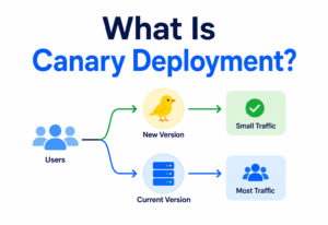
This staged rollout matters more for an ML-driven system than for typical stateless services, because a bad model deployment does not crash loudly — it degrades quietly, making subtly worse decisions that might not be obvious until real business impact shows up days later. Canary rollout with automatic rollback closes that gap by comparing live metrics against the previous model in near real time, not just at deploy time.
Infrastructure as code
Given how many independently scaled components this system has (event gateway, stream processing cluster, feature store shards, scoring replicas, decision service), managing them by hand quickly becomes unmanageable. Defining the entire topology declaratively (Terraform for cloud resources, Helm charts for Kubernetes workloads) makes the environment reproducible and makes standing up an entire second region for disaster recovery a matter of running the same definitions elsewhere.
Rolling back safely, quickly and without ambiguity
A rollback for this system is not just redeploying old code — it is reverting to a previous model artifact and it needs to happen fast enough to matter during an active incident. Keeping the previous several model versions readily available in the registry, rather than only the current one and keeping the Scoring Service capable of hot-swapping between registered model versions without a full redeploy, turns a rollback from a multi-minute deployment pipeline run into a near-instant configuration change. Practicing this rollback path deliberately, before it is ever needed under real pressure, is what separates a rollback that takes seconds from one that takes twenty stressful minutes while a bad model is actively making poor decisions in production.
“Why go through shadow deployment and canary rollout instead of just A/B testing model versions?” A good answer distinguishes the two: A/B testing measures business impact on live users deliberately exposed to a change, which is appropriate once you already trust the model is safe; shadow and canary are safety gates that come before that, designed to catch a badly broken model before it ever influences a real decision.
Patterns & Anti-patterns
Patterns worth reusing
CQRS-style split
Writes (engagement events) and reads (feature lookups, scoring) go through entirely different paths optimised independently, rather than one shared model trying to serve both well.
Circuit breaker
Every synchronous call between services (e.g. Scoring Service → Feature Store) is wrapped so a slow dependency degrades gracefully instead of cascading failure upstream.
Shadow deployment
New models prove themselves against live traffic before ever influencing a real decision — covered in Sections 6 and 14.
Event sourcing
The commit log of raw engagement events is the true source of truth; every derived table or cache (feature store, aggregates) can be rebuilt from it if needed.
Anti-patterns to avoid
Fixed global thresholds
As discussed in Section 1, a single hard-coded velocity threshold fails across account sizes, content categories and regions. Thresholds should be learned or at least segmented, never one constant for the whole platform.
Synchronous scoring on the write path
Coupling event ingestion directly to a model inference call blocks the fast path (which needs to stay cheap and simple) behind the slow path (which is inherently more expensive) and makes ingestion fragile to model-serving issues.
Training on today’s data, deploying tomorrow, evaluating never
Skipping the shadow / canary safety net because “the offline metrics looked good” is how silent regressions reach production undetected.
Treating engagement counts as trustworthy by default
Ignoring manipulation detection (Section 12) until it becomes a visible problem, rather than building it in as a first-class feature category from the start.
The bulkhead pattern applied to per-post load
Borrowed from ship design, where watertight compartments keep a single hull breach from sinking the entire vessel, the bulkhead pattern isolates resource pools so that one overloaded consumer cannot starve every other consumer of shared capacity. Applied here, this means a single extraordinarily hot post should be prevented from monopolising the thread pool or connection pool that the Scoring Service uses for every other, ordinary post being scored at the same moment. Dedicating a small, separate pool of capacity specifically for the handful of posts already confirmed to be trending — the ones Section 10 discussed adaptively sampling — keeps a viral spike from degrading the experience for the much larger number of posts still in normal processing.
Why a strangler-fig migration path matters for a system like this
Very few teams build a system exactly like this one from a blank slate — more often, it evolves out of a simpler existing trending or ranking system that already has real production traffic and real stakeholders depending on it. The strangler-fig pattern — routing an increasing share of traffic to the new pipeline while the old one keeps running unchanged, until the old system can be safely retired — is usually the more realistic path than a single cutover, precisely because it lets the new prediction-based approach be validated against real outcomes, side by side with the previous approach, before anyone has to commit fully to it.
“What is the biggest architectural mistake teams make building a system like this?” A thoughtful answer usually lands on coupling ingestion too tightly to scoring — treating this as one monolithic “engagement pipeline” rather than clearly separated ingestion, feature computation, scoring and decision stages, each with different scaling and reliability needs.
Best Practices & Common Mistakes
Best practices
- Design the feature set to be interpretable, not just accurate — every score should be explainable in terms of a handful of named features, which matters enormously for trust and safety review and for debugging model behaviour.
- Build the cold-start heuristic before the full ML model, not after. It defines the floor of acceptable behaviour and gives you a safe fallback from day one rather than as an afterthought.
- Treat decision thresholds as configuration, not code — different downstream consumers (recommendation vs. trust & safety) legitimately want different sensitivity and hard-coding one threshold forces an awkward compromise.
- Instrument precision and recall against resolved outcomes from the very first production deployment, even if the model is simple — you cannot improve what you never started measuring.
Common mistakes
- Optimising purely for recall (catching every viral post) without accounting for the operational cost of false positives, which quietly erodes trust in the system among the teams consuming its decisions.
- Letting the stream processor’s windowing logic silently diverge from the offline feature computation used for training — a subtle mismatch here (sometimes called training-serving skew) is one of the most common, hardest-to-debug sources of poor real-world model performance.
- Under-investing in the event gateway’s validation logic, on the assumption that “it is just logging a like” — malformed or spoofed events poison every downstream feature silently.
- Forgetting that “viral” is a moving target — what counts as an outlier engagement rate changes over time as the platform itself grows, so labels and thresholds need periodic recalibration, not a one-time definition.
Building for the team that inherits this system, not just the team that ships it
A subtler best practice worth naming explicitly: a real-time ML system like this one tends to outlive the engineers who originally built it and design decisions that felt obvious at launch time can be genuinely mysterious to whoever operates it two years later. Documenting why a threshold was set where it was, why a particular feature was included and why a given fallback behaviour was chosen — not just what the current values are — pays off enormously during an incident at 2 a.m. when the person on call is someone who never sat in on the original design discussion. The interview callouts and analogies used consistently throughout this guide reflect that same instinct: a system is only as maintainable as the reasoning behind it is discoverable to the next person who needs to change it.
This deserves its own callout because it is genuinely one of the most common real-world failures in systems like this. If the stream processor computes “velocity_5m” using a slightly different windowing rule than the offline batch job that generates training data, the model learns patterns that do not actually exist in production and performance degrades in ways that are very hard to diagnose from metrics alone. The fix is architectural: compute features with the exact same code path for both training and serving wherever possible, rather than maintaining two separate implementations.
Algorithms, Consistency & Cost
A few deeper technical questions tend to come up once the high-level architecture is settled: what data structures actually make the windowed counting cheap at scale, how much consistency does this pipeline really need and what does running it cost. This section works through all three.
Counting uniques cheaply: HyperLogLog
The unique_user_ratio feature from Section 5 requires knowing, for every active post, roughly how many distinct users engaged with it — but storing an exact set of user IDs per post, per time window, becomes expensive fast when there are millions of posts active at once and some individual posts have millions of engagers. This is exactly the situation a probabilistic data structure called HyperLogLog was built for. Instead of storing every user ID, it stores a small, fixed-size sketch (a few kilobytes, regardless of whether the true count is a hundred or a hundred million) and estimates the distinct count from that sketch with a small, well-understood error margin, typically under two percent. For a feature that only needs to distinguish “engagement came from thousands of different accounts” from “engagement came from twenty accounts liking repeatedly”, that error margin is entirely acceptable and the memory savings make sharded, per-post, per-window unique counting practical at all.
Imagine trying to estimate how many distinct people are in a stadium by looking at the highest row number anyone is sitting in, rather than counting every single seat individually. It is a strange-sounding trick, but with the right statistical adjustment it gives a surprisingly accurate estimate using almost no information — that is the same basic spirit behind HyperLogLog, just applied to the pattern of bits in a hashed user ID instead of seat numbers.
Counting approximate frequencies: Count-Min Sketch
A related problem shows up when trying to detect whether engagement on a post is unusually concentrated among a small number of accounts — a useful manipulation signal from Section 12. Rather than maintaining an exact frequency table of every user who has engaged with every post, a Count-Min Sketch provides an approximate frequency count using a small, fixed amount of memory and a handful of hash functions, trading a controlled amount of over-counting error for a massive reduction in memory footprint. Both of these sketches share a common theme worth remembering for system design discussions generally: when a system needs to track a statistic across a huge number of independent keys (here, posts) in bounded memory, exact data structures often are not the right tool — approximate, sketch-based structures usually are.
Sliding window computation without recomputing everything
Naively, computing a 30-minute sliding window average by re-summing all events in that window on every update would mean the cost of each update grows with the window size. Real stream processors avoid this using a technique sometimes called a sliding window aggregator: maintain the current windowed sum incrementally, adding new events as they arrive and subtracting expired events as they age out of the window, so each update is constant-time regardless of how large the window is. This is the same underlying idea as a two-pointer or deque-based sliding window technique from classic algorithms — the stream processing engine is really just applying that pattern continuously, per key, across millions of keys in parallel.
How much consistency does this pipeline actually need?
It is worth being explicit about where this system sits on the CAP theorem’s consistency-versus-availability spectrum, because the answer is different for different parts of the pipeline and conflating them leads to over-engineering in some places and under-engineering in others.
| Component | Consistency model | Why |
|---|---|---|
| Kafka event log | Strong ordering per partition, eventual replication across brokers | Losing strict global ordering across all posts is fine; losing ordering of one post’s own events would break windowed aggregation |
| Hot feature store | Eventually consistent, tolerant of a few seconds of staleness | A feature read that is two seconds stale barely changes a virality score; waiting for strong consistency here would add latency for no real benefit |
| Decision idempotency store | Strongly consistent, read-your-writes | Preventing a duplicate promotion decision (Section 9) genuinely requires a correct, immediate check-and-set — this is the one place strong consistency earns its cost |
| Cold storage / data lake | Eventually consistent, batch-oriented | Training data can tolerate minutes of replication lag with no practical downside |
This table is a useful template for almost any real-time system design discussion: rather than answering “is this system CP or AP” as one global choice, decompose it component by component and justify each choice against what actually breaks if consistency is relaxed there.
Consensus underneath the stream bus
Kafka’s own durability guarantees rest on a consensus protocol among its brokers (historically ZooKeeper-based, increasingly self-managed via KRaft in modern deployments) to agree on partition leadership and commit offsets safely even when individual brokers fail. This system does not need to reimplement consensus — it inherits correctness guarantees from the stream bus underneath it — but it is worth being able to explain, at a high level, why a leader-based replication scheme with a quorum write requirement is what allows the system to promise “an acknowledged event will not be lost”, which is the durability foundation everything else in this guide quietly depends on.
Failure recovery in the stream processor
Stream processing frameworks like Flink checkpoint their internal state (the in-progress windowed aggregates) periodically to durable storage. If a processing node crashes mid-window, it does not lose the partial aggregate for every post it was tracking — it resumes from the last checkpoint and replays the small number of events since that checkpoint from Kafka, using the offsets Kafka already durably tracks. This checkpoint-and-replay pattern is what makes the windowed features in Section 5 resilient to individual node failures without needing to synchronously replicate every state update, which would be far more expensive.
Cost optimisation
A system that continuously scores every active post can get expensive quickly if left unchecked and a few deliberate trade-offs keep the cost proportional to actual value delivered rather than to raw traffic volume.
- Tiered scoring frequency: brand-new posts are scored every few seconds, since that is when the “before it happens” advantage is most valuable; posts that have been flat for an hour are scored on a much slower cadence, since their trajectory rarely changes suddenly at that stage.
- Sketch-based structures over exact ones: as covered above, HyperLogLog and Count-Min Sketch are not just an elegant algorithmic choice — replacing exact per-post user sets with small fixed-size sketches is a direct, measurable infrastructure cost reduction at scale.
- Cold storage tiering: raw event data older than a defined window moves from more expensive hot object storage to cheaper archival storage tiers automatically, since training pipelines need statistically representative history far more than they need the single most recent minute of data to be instantly accessible.
- Right-sizing the model: a smaller gradient-boosted tree model that runs cheaply on CPU at high volume is very often the better economic choice over a larger deep model that requires GPU serving, unless the accuracy gain from the larger model can be shown to justify the added infrastructure cost in real business terms.
“Your unique-user-count feature is becoming a memory bottleneck at scale. What would you do?” This is a natural opening to bring up HyperLogLog specifically: explain the trade-off being made (a small, bounded estimation error in exchange for a large, fixed reduction in memory per key) and note that this class of trade-off — approximate but cheap versus exact but expensive — comes up constantly in large-scale systems, not just this one.
Industry Case Studies
The following describes, in general terms, how this class of problem is approached across the industry — the specific implementation details of any single company’s proprietary system are not public, but the broad architectural patterns are well known and widely discussed.
It is worth noting up front that no two platforms weight the same signals identically, even when they are solving what looks like the same underlying problem, because the definition of “good” content and the shape of a healthy engagement curve differ meaningfully by product. A platform built around short, disposable content and one built around durable, long-shelf-life content will naturally define virality and therefore build their feature sets and thresholds, quite differently — even while sharing the same underlying pipeline shape described throughout this guide.
Short-video platforms
Short-video platforms lean especially heavily on early watch-time and completion-rate signals rather than likes or shares alone, because a video that gets watched all the way through repeatedly in its first hour is one of the strongest known predictors of broader distribution — arguably more predictive than any single explicit engagement action, since it is much harder to fake passively.
Social / text platforms
Text-and-link-sharing platforms put more relative weight on network diversity signals — whether a post is spreading across otherwise-unconnected communities rather than staying within one densely connected group — since that pattern strongly distinguishes organic virality from a coordinated push within a single community.
Marketplaces & review platforms
Platforms centred on reviews or user-generated recommendations apply similar velocity-and-acceleration thinking to a different unit: instead of predicting whether a single post goes viral, they predict whether a specific product or listing is about to see a sustained demand spike, using much the same architecture — event stream, windowed features, a scoring model — applied to a different entity type.
Livestreaming & real-time events
Livestreaming platforms face a variant of this problem with an even tighter time budget: a stream that is about to be “raided” by a large audience from another stream, or a moment within an ongoing broadcast that is about to be widely clipped and shared, needs to be detected while the stream is still live for any intervention to matter at all. This pushes the architecture from this guide toward even shorter windows and a heavier reliance on the cold-start heuristic style of reasoning from Section 6, since there is often no time to wait for the fuller, more data-hungry model to become confident before the moment has already passed.
News and information platforms
Platforms centred on news and current-events content have an additional wrinkle: virality here is often tightly coupled to external, real-world events rather than purely to the content’s own intrinsic qualities. A modest news item can go viral extremely fast purely because it relates to a breaking real-world story, independent of anything about how the post itself was written or produced. Systems in this space commonly incorporate an external signal feed — spikes in web search interest, or a surge of activity across many unrelated posts referencing the same real-world entity — as an additional early feature, supplementing the purely engagement-based features covered in Section 5 with a form of external context that a purely internal-signal system would miss entirely.
Common thread across all of them
Despite different products and different specific features, the underlying architecture converges on the same shape covered throughout this guide: a durable event stream, windowed real-time feature computation decoupled from raw events, a lightweight and fast-serving model and a continuous retraining loop grounded in real outcomes. That convergence is a strong signal that this is close to the right general shape for this class of problem, independent of the specific platform.
“Would this architecture change much if you were predicting viral products in an e-commerce marketplace instead of viral social posts?” The right instinct is: surprisingly little at the architectural level — swap “post” for “listing” and adjust the specific feature set, but the ingestion → windowed features → scoring → decision spine stays the same. Recognising that the architecture generalises is more valuable than memorising platform-specific details.
Frequently Asked Questions
Q: How early can this system realistically detect virality?
It depends heavily on content type and audience size, but well-tuned systems commonly produce a useful signal within the first 15–60 minutes of a post’s life — well before it would be obvious to a human scrolling a feed, though rarely in the first few minutes, where data is simply too thin to be reliable (the cold-start problem from Section 2).
Q: Is this the same thing as a trending-topics algorithm?
They are related but distinct. A trending-topics algorithm typically surfaces what is already popular right now, aggregated across many posts on a theme. A virality detection system predicts the future trajectory of individual pieces of content, often before they are popular enough to register as trending at all.
Q: Does this require deep learning?
Not necessarily. As covered in Section 6, gradient-boosted trees on well-engineered tabular features are a strong, efficient starting point and are what many production systems actually run. Deep learning becomes more valuable specifically when raw content — text, image, or video — is incorporated directly rather than only behavioural signals.
Q: How do you avoid the system becoming a self-fulfilling prophecy — promoting content that then goes viral only because it was promoted?
This is a genuine, well-known challenge for any system that both predicts and influences outcomes. One mitigation is holding out a small, randomised control group of posts that meet the flagging criteria but are deliberately not promoted, purely to measure what would have happened organically — a technique borrowed from causal inference that keeps the training data honest.
Q: What is the single hardest part of building this in practice?
Most practitioners point to the same thing: getting reliable ground-truth labels. “Did this post actually go viral” sounds simple but requires a precise, consistently applied definition (Section 2) applied consistently over time as the platform itself grows and baseline engagement shifts.
Q: Can this system work for a small platform without Kafka-scale infrastructure?
Yes and it is worth designing for that explicitly. The same five-stage shape — ingest, aggregate, score, decide, retrain — works with far simpler technology at smaller scale: a managed queue instead of a self-hosted Kafka cluster, a single relational database with a well-indexed events table instead of a tiered storage system and a simpler heuristic instead of a full gradient-boosted model. The architecture should grow into the more elaborate version described throughout this guide as traffic actually demands it, not be built at full scale on day one.
Q: How do you handle content in multiple languages or regions with very different baseline engagement patterns?
The creator-baseline and category-baseline features from Section 5 need to be segmented by region and, where relevant, by language, rather than computed globally. A post’s engagement velocity that would be extraordinary in a smaller regional market might be entirely ordinary in the platform’s largest market, so the statistical baseline the model compares against has to reflect the right comparison group, not a single global average.
Q: Should the model be retrained continuously, or on a fixed schedule?
Most production systems land on a fixed, fairly frequent schedule — daily or a few times a week — rather than truly continuous online learning, because the evaluation and safety gates from Sections 6 and 14 (shadow deployment, canary rollout) take real time to run properly and rushing a new model into production without them defeats the purpose of having them. Continuous retraining without continuous evaluation is a common source of the silent regressions discussed in Section 16.
Summary & Key Takeaways
Key takeaways
- Virality detection reframes a backward-looking measurement problem (“what went viral”) as a forward-looking prediction problem (“what is about to”), which is what makes it valuable and what makes it hard.
- The core architecture is a five-stage pipeline: ingest engagement events on a durable stream, compute windowed features that capture velocity and acceleration, score those features with a fast model, apply business rules in a separate decision layer and continuously retrain on real outcomes.
- Feature engineering — not the model algorithm — is where most of the real difficulty and most of the value live. Velocity, acceleration, unique-reach and audience diversity matter more than raw engagement counts.
- Cold-start handling, graceful degradation and shadow / canary deployment are not optional extras — they are what keeps an ML-driven real-time system trustworthy under the exact high-load conditions it exists to handle.
- The same architectural shape generalises well beyond social content — to product demand spikes, trending searches, or any domain where early behavioural signals predict a future surge.
- None of the individual pieces here — stream processing, gradient-boosted trees, probabilistic sketches, canary deployments — are exotic on their own. What makes this system genuinely interesting to design is how tightly the time budget across every stage constrains the choices available and how much of the real engineering effort goes into graceful degradation, safety gates and explainability rather than into the prediction algorithm itself.
The seismograph analogy from Section 1 is worth returning to. A good virality detection system, like a good seismograph, is not trying to be impressive — it is trying to be quietly, consistently right just often enough, just early enough, that by the time everyone else notices the spike, the system has already moved on to watching the next one.