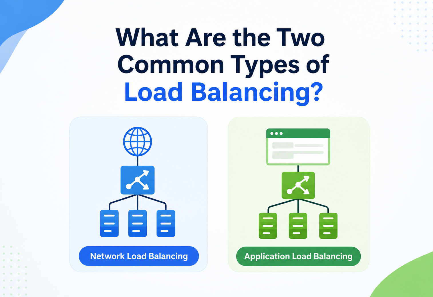
What Are the Two Common Types of Load Balancing?
Every load balancer, every time a new request arrives, has to answer a single deceptively simple question: which server should handle this one? The two most fundamental families of answers — static load balancing (which follows a fixed plan) and dynamic load balancing (which watches the servers in real time) — are what this complete guide is about. Together, they cover almost every well‑known algorithm you will ever meet.
The Big Idea, in One Breath
Load balancers face the exact same fork in the road every single time a new request shows up. Either they follow a fixed plan, or they check the room first and decide accordingly. Those two paths have names: static and dynamic.
Picture a teacher handing out worksheets to a classroom of thirty kids. There are two completely different ways to go about it. The teacher could simply walk down each row, giving one worksheet to each student in the exact same order every single day — first row first, second row second, always the same pattern, no matter who finished yesterday’s worksheet quickly and who is still struggling with it.
Or, the teacher could actually glance around the room first, notice which students already have their hands free and which ones are still buried in other work, and hand the next worksheet to whoever looks genuinely ready for it. The first approach is fast, predictable, and requires zero thinking. The second approach takes a little more effort and attention, but it results in a much fairer, smoother classroom where nobody sits idle while someone else drowns in work.
Load balancers face this exact same fork in the road every single time a new request shows up, and the two paths they can choose between are known as static load balancing and dynamic load balancing. These are, by a wide margin, the two most fundamental and most commonly discussed types of load balancing in the entire field, and understanding the difference between them unlocks almost everything else worth knowing about how traffic gets shared out fairly across a group of servers.
Imagine two ice cream trucks working a busy summer fair. The first truck’s owner always parks in the exact same spot, every single day, whether the fair is packed or nearly empty. The second truck’s owner walks the fairgrounds first, notices where the biggest crowd is gathering that particular day, and parks right there instead. Both trucks sell ice cream. Only one of them is actually paying attention to what is happening right now.
What “Types” Actually Means Here
Before going any further, it is worth being precise about exactly what question this guide is answering, because the word “type” gets used loosely in load balancing conversations.
People sometimes use “type of load balancer” to mean hardware versus software, or Layer 4 versus Layer 7, or local versus global — all genuinely useful ways of categorising load balancers, but each one is answering a different question.
This guide is focused specifically on the classification that sits underneath the actual decision‑making logic — the algorithm a load balancer follows to pick a server for each incoming request. When people ask “what are the two common types of load balancing,” they are almost always asking about this exact split: does the decision‑making follow a fixed, unchanging pattern, or does it adapt based on what is actually happening on the servers right now? That question sorts every well‑known load balancing algorithm into exactly one of two buckets, and those two buckets are the heart of this entire guide.
Think of “static versus dynamic” as answering the question “does the load balancer look before it leaps?” A few other useful classifications exist too, and this guide covers them briefly near the end, but the static‑versus‑dynamic split is the one most people mean when they ask this exact question.
This particular classification also happens to be the one taught first in nearly every system design course and technical interview preparation guide, and for good reason: it is the split that most directly shapes how a load balancer actually behaves under real, changing conditions. Understanding hardware versus software tells you where a load balancer physically lives. Understanding Layer 4 versus Layer 7 tells you how much of a request it can see. Understanding static versus dynamic tells you whether it is paying attention at all — arguably the single most consequential question of the bunch.
The Two Types at a Glance
Before diving into individual algorithms, it helps enormously to see the whole picture laid out side by side. Every specific method covered in this guide is really just one particular flavour sitting underneath one of these two broad umbrellas.
Notice, too, that within each family, the individual algorithms are not scattered randomly — they form a gentle progression, each one adding a small refinement on top of the one before it. Round robin gets refined by weighting; least connections gets refined the very same way. This shared pattern is worth keeping in the back of your mind as this guide walks through each algorithm individually over the next several sections, since it turns nine separate names into what is really just two simple ideas, each explored a little more deeply.
Static Load Balancing Explained
Static load balancing follows a fixed, predetermined pattern to decide which server gets each request, without ever checking how busy, healthy, or fast any particular server is at that moment.
The rules are decided ahead of time, written down, and then followed mechanically, request after request, completely unaware of anything happening on the servers in real time.
This might sound like a weakness at first glance, and in certain situations it genuinely can be. But there is real elegance hiding in that simplicity. A static algorithm does not need to constantly ask each server “how are you doing?” before making a decision, which means it can make that decision almost instantly, with barely any extra computing effort spent on the decision itself. For a pool of servers that are all roughly identical in power and generally healthy, this simplicity is not a compromise at all — it is often exactly the right amount of sophistication for the job.
Almost no overhead
No time spent checking server status means the routing decision itself happens about as fast as physically possible.
Easy to set up and debug
Fewer moving parts means fewer places for something to quietly go wrong, and troubleshooting stays refreshingly straightforward.
Behaves the same way, always
Given the same sequence of requests, a static algorithm will make the exact same choices every single time.
Cannot see trouble brewing
A server quietly struggling under heavy load still receives its “fair share” of new requests, making the struggle worse.
It is worth being precise about what “static” does and does not mean here. It does not mean the configuration can never be changed by a human — an engineer can absolutely go in and adjust weights or reorder the list whenever they like. What makes it “static” is that the load balancer itself never makes that adjustment automatically, in the moment, based on what it is observing. The plan only changes when a person deliberately changes it.
Round Robin
Round robin is, without much competition, the most famous and most widely used static algorithm in existence — and often the very first one anyone learns. The load balancer keeps a simple list of available servers and hands out incoming requests one after another, straight down that list: the first request to the first server, the second to the second server, and so on. Once the bottom of the list is reached, it simply loops back around to the top and starts again.
Where It Shines
- Wonderfully simple to configure and understand.
- Guarantees perfectly even request counts over time.
- Ideal when every server has near‑identical power.
Where It Struggles
- Ignores whether a server is already overwhelmed.
- Treats a powerful server the same as a weak one.
- Does not account for requests that take vastly different amounts of time.
Round robin works beautifully as long as its core assumption holds true: that every server is roughly equal, and every request takes roughly the same amount of effort to answer. The moment either of those assumptions breaks down — say, one server is noticeably weaker, or some requests are far heavier than others — round robin can quietly start creating exactly the kind of imbalance it was supposed to prevent.
Round robin’s name actually comes from an old letter‑writing tradition, where a group of people would pass a single letter around in a circle, each person adding their own note before passing it to the next — a fitting origin for an algorithm whose entire personality is “everybody gets an equal, orderly turn.” That same spirit of fairness‑by‑rotation is exactly why round robin remains the algorithm most people picture first when they hear the phrase “load balancing” at all.
Weighted Round Robin
Weighted round robin takes the familiar round robin pattern and adds one clever adjustment: instead of every server getting an identical turn, each server is assigned a weight — a number reflecting how much traffic it can realistically be trusted to handle. A server given a weight of three effectively receives three requests for every single request sent to a server with a weight of one.
This small tweak solves round robin’s biggest blind spot in one elegant move: it lets a pool of genuinely mismatched hardware — a newer, more powerful server sitting alongside an older, weaker one — still be shared out fairly, in proportion to what each machine can actually handle, rather than pretending they are all equally capable.
Weighted round robin is especially handy during a gradual server upgrade, when a company is running a mix of old and new hardware side by side and wants new, more powerful machines to shoulder a bigger share of the load without retiring the older ones early.
The one thing weighted round robin still does not do is glance at real‑time conditions. Even a heavily weighted, powerful server can occasionally hit a rough patch — a slow database query, a memory spike — and weighted round robin has no way of noticing or reacting to that in the moment. It is a smarter fixed plan, but it is still, at its core, a fixed plan.
Choosing the right weight for each server is itself a small skill worth mentioning. Weights are sometimes set once, based on a server’s specifications on paper, and never revisited — a habit that can quietly go stale as hardware ages or gets upgraded. A more careful approach revisits weights periodically, informed by actual observed performance rather than the numbers printed on a spec sheet years earlier.
Random Distribution
Sometimes the simplest possible idea turns out to be surprisingly effective. The random algorithm does exactly what its name suggests: each new request is handed to a server chosen essentially by chance, with no fixed order and no memory of who received the last request.
Over a very large number of requests, pure randomness tends to average out into something close to an even spread — not because any single decision was carefully planned, but simply because the law of large numbers works quietly in the background. For a pool of similarly powered servers handling a high, steady volume of requests, random distribution can perform nearly as well as round robin, with the added benefit of being even simpler to implement, since there is no list position to keep track of at all.
Where It Shines
- Extremely simple, with almost nothing to configure.
- No need to track any ongoing state or position.
- Averages out reasonably well over high volumes.
Where It Struggles
- Short‑term imbalance is entirely possible by pure chance.
- Offers no guarantee of fairness over a small number of requests.
- Still completely blind to real server conditions.
It is a little counterintuitive that “pure chance” can hold its own against a carefully ordered rotation, but the comparison highlights something worth remembering throughout this entire guide: simplicity and effectiveness are not opposites. Random distribution is proof that a load‑balancing method does not need to be clever to be genuinely useful — it just needs to match the actual shape of the problem it is solving.
Source IP Hash
The source IP hash algorithm takes a very different approach from anything covered so far. Instead of cycling through servers or picking one at random, it runs the visitor’s own IP address through a mathematical formula called a hash function, and the result consistently points to the exact same server, every single time that same visitor sends a request.
This consistency is the entire point. Some applications genuinely need a particular visitor to keep talking to the same server across multiple requests — perhaps that server is holding onto some temporary information about the visitor’s current session. Source IP hash provides this consistency without needing cookies or any extra coordination between servers; the math itself guarantees the outcome.
If the one server a visitor keeps getting hashed to happens to go down, that visitor can experience real disruption until the server comes back — or until the hashing recalculates and reassigns them elsewhere. Consistency and resilience sit in gentle tension here.
It is worth noting that source IP hash is not quite as perfectly reliable as it might first sound, especially in modern networks. Many visitors on the same shared office network, or behind the same mobile carrier, can appear to a server as coming from the exact same IP address, which can accidentally funnel a disproportionate crowd toward a single server. This is one reason many modern systems prefer solving the “remember this visitor” problem with cookies or shared session storage instead, reserving IP hashing for narrower situations where it is genuinely the best fit.

URL Hash
URL hash works on the same underlying principle as source IP hash, but it looks at a different piece of information: the specific web address, or URL, being requested, rather than who is asking for it. The load balancer runs the URL itself through a hash function, and the result consistently points requests for that exact URL toward the same server every time.
This turns out to be especially useful when different servers in a pool specialise in different kinds of content rather than being fully interchangeable copies of each other. If one group of servers holds cached product images and another handles checkout logic, URL hashing can reliably send “give me this product photo” requests toward the servers that already have that image ready and waiting, rather than spreading that request randomly across servers that would each have to fetch it fresh.
Because the same URL keeps landing on the same server, that server has a much better chance of already having a cached, ready‑to‑go answer sitting in memory — turning a routing decision into a free performance boost as well.
URL hashing shares a family resemblance with source IP hashing — both rely on the same underlying trick of turning a piece of information into a consistent, repeatable server choice — but they solve genuinely different problems. Source IP hashing cares about who is asking; URL hashing cares about what is being asked for. A single system occasionally uses both together, layered at different points, when both kinds of consistency happen to matter at once.
Dynamic Load Balancing Explained
Dynamic load balancing checks the current state of each server — how busy it is, how healthy it is, how quickly it has been responding — before deciding where to send each new request, adjusting its behaviour continuously as those conditions change.
Rather than following a script written in advance, it is constantly re‑reading the room.
This awareness does not come for free. Dynamic algorithms need some kind of ongoing communication between the load balancer and each server — a steady trickle of information about connection counts, response times, or available resources — and processing all of that information takes a little extra time and computing effort compared to simply following a fixed list. For anything beyond a small, simple, uniform pool of servers, though, that small cost is very often worth paying many times over.
Adapts to real conditions
A server that is quietly struggling receives less new work, instead of getting piled on regardless.
Notices trouble quickly
Slowdowns and partial failures get factored into decisions almost as soon as they happen.
More to configure
Requires ongoing monitoring, communication, and tuning that a static setup simply does not need.
A small, worthwhile cost
Extra computation is spent making each decision, in exchange for a noticeably smarter outcome.
It is worth noting that “dynamic” comes in degrees rather than being a single, fixed level of sophistication. Least connections is dynamic, but only in a fairly narrow sense — it watches one specific number. Resource‑based balancing is dynamic in a much deeper sense, watching several different signals at once. As this guide moves through the specific dynamic algorithms next, notice how each one adds just a little more awareness than the one before it.
Least Connections
Least connections is the most intuitive and widely used dynamic algorithm, and it is a natural first step beyond the static world. The load balancer keeps track of how many active connections each server currently has open, and every new request gets sent to whichever server currently has the fewest.
This method is particularly valuable whenever connections stick around for a while rather than finishing instantly — think live chats, file transfers, or long‑running database queries. In these situations, a simple round‑robin count of “how many requests has each server received today” tells you very little about how busy a server actually is right now, because some of those earlier connections might still be wide open, quietly consuming resources.
Where It Shines
- Naturally adapts to genuinely uneven workloads.
- Especially strong with long‑lived, persistent connections.
- Prevents any one server from being silently buried.
Where It Struggles
- Assumes every connection needs roughly equal effort.
- Adds a small ongoing bookkeeping cost to the load balancer.
- Can be fooled by many short, cheap connections stacking up.
Least connections marks an important turning point in this guide, because it is the first algorithm covered that genuinely requires a two‑way relationship between the load balancer and the servers it manages. Static methods only ever need to know the list of servers that exist; least connections needs a constant, quiet stream of updates about what those servers are currently doing. That extra relationship is exactly what “dynamic” means in practice, not just in theory.
Weighted Least Connections
Just as weighted round robin improved on plain round robin, weighted least connections improves on plain least connections by acknowledging that not all servers can comfortably handle the same number of simultaneous connections. Each server is given a capacity rating, and the load balancer compares each server’s current connection count against that capacity, rather than comparing raw numbers alone.
In practice, this means a powerful server carrying eighty open connections might still be considered “less busy” than a modest server carrying only twenty, if the powerful server’s rated capacity is proportionally much higher. This blending of real‑time awareness with known hardware differences makes weighted least connections one of the more balanced, practical choices for a mixed pool of servers under genuinely variable load.
Think of weighted least connections as asking not “who has the fewest connections?” but “who has the most comfortable room left, relative to what they are actually built to handle?” — a subtly fairer question.
This method tends to show up in mature systems that have already grown past their original, uniform hardware — a company that started with five identical servers and, over time, added newer, stronger machines rather than replacing everything at once. Weighted least connections lets that gradually growing, gradually mismatched pool keep working fairly together, without forcing an expensive, disruptive hardware refresh just to keep the load balancing logic simple.

Least Response Time
Least response time pushes the idea of “watching the servers” one step further still. Rather than only counting active connections, it also tracks how quickly each server has actually been answering recently, and combines both pieces of information to make its decision.
This distinction matters because connection count alone can occasionally be misleading. A server might have very few open connections yet still be answering unusually slowly, for reasons that have nothing to do with connection count at all — perhaps it is running a background task, or struggling with a slow disk. Least response time catches exactly this kind of hidden trouble, steering new traffic away from a server that is technically “not busy” by the numbers but is quietly underperforming in practice.
Where It Shines
- Catches subtle slowdowns that connection counts alone would miss.
- Rewards genuinely fast, healthy servers with more traffic.
- Tends to produce noticeably snappier overall performance.
Where It Struggles
- Requires ongoing timing measurements, adding complexity.
- A brief, unusual delay can temporarily and unfairly penalise a good server.
- More moving parts than simpler dynamic methods.
Many production load balancers soften that last weakness by looking at response times measured over a short rolling window — say, the last thirty seconds — rather than reacting instantly to a single slow reply. This small smoothing trick prevents one unlucky, momentary blip from unfairly branding an otherwise excellent server as “slow” and starving it of new traffic for longer than it deserves.
Resource‑Based Balancing
Resource‑based balancing is the most thorough and detailed dynamic approach commonly used today. Rather than inferring how busy a server is from connection counts or response times alone, it goes straight to the source: a small helper program running on each server reports back real, live information about that server’s actual processing power and memory currently in use.
The load balancer uses this direct, honest snapshot — rather than an indirect guess — to decide where new work should go, checking that a server genuinely has free capacity before sending it anything new. This is, in a real sense, the dynamic family’s philosophy taken to its logical conclusion: instead of guessing at how busy a server is through secondhand clues, simply ask it directly and act on the answer.
This depth of insight comes with the highest setup cost of any method covered in this guide — it requires installing and maintaining that small reporting program on every server in the pool. For systems where server health can vary in subtle, hard‑to‑predict ways, that investment often pays for itself many times over.
Resource‑based balancing is often the method of choice for large, mixed workloads where different requests genuinely consume wildly different amounts of processing power or memory — think of a platform that handles both simple lookups and heavy, resource‑intensive computations side by side. In that kind of environment, connection counts and response times alone can miss the real story, and only a direct look at actual resource usage gives the load balancer the full picture it needs to make a genuinely well‑informed decision.
Side‑by‑Side Comparison
With all nine algorithms now on the table, it is worth stepping back and comparing the two families directly, one important dimension at a time.
| Dimension | Static | Dynamic |
|---|---|---|
| Awareness of server load | None | Continuous |
| Setup complexity | Low | Moderate to high |
| Decision speed | Extremely fast | Fast, with a small overhead |
| Behaviour with mismatched servers | Can be unfair, unless weighted | Naturally adapts |
| Behaviour during a slowdown | Keeps sending traffic regardless | Automatically sends less |
| Best fit | Small, uniform, predictable pools | Larger, variable, unpredictable pools |
Neither column is objectively “the winning one.” A small internal tool running on three identical servers gains very little from the added complexity of dynamic balancing. A large, public‑facing platform juggling unpredictable traffic across dozens of differently sized servers, on the other hand, would likely struggle badly if it stuck with a purely static approach. The right choice depends entirely on the shape of the actual problem in front of you.
Performance Impact in Practice
It helps to ground all of this in what actually changes, numbers‑wise, when a system switches from a static to a dynamic approach. The honest answer is: it depends heavily on how uneven the underlying servers and requests really are.
On a genuinely uniform pool of servers handling genuinely uniform requests, switching from round robin to a dynamic method typically produces only a marginal improvement, because there was very little unevenness to correct in the first place — while still adding a small, measurable amount of extra decision‑making overhead. The story flips dramatically, though, the moment real unevenness enters the picture. On a mismatched pool handling wildly different request sizes, a dynamic method can meaningfully reduce how often any single server gets overwhelmed, often translating into noticeably fewer slow responses and timeouts during genuine traffic spikes.
This is exactly why blindly benchmarking “static versus dynamic” in the abstract, without reference to a specific real system, tends to produce misleading advice. The honest, useful question was never “which one is faster in general” — it was always “how uneven is my particular situation, and does that unevenness justify the small extra cost of watching more closely?”

How to Choose Between Them
Rather than defaulting to whichever option sounds more impressive, a sensible choice usually comes down to answering a small handful of honest questions about the actual system in front of you.
Are your servers roughly equal in power?
If yes, plain round robin or random distribution may already be perfectly adequate.
Are your servers meaningfully different in capacity?
Reach for a weighted static method first, before jumping straight to full dynamic complexity.
Does traffic swing unpredictably?
Unpredictable, bursty, or highly variable traffic is exactly where dynamic algorithms start earning their keep.
Do requests vary hugely in how much work they cause?
If some requests are trivial and others are heavy, connection‑ or response‑time‑aware methods pay off quickly.
Can your team realistically maintain extra complexity?
A dynamic setup nobody fully understands can become its own source of mysterious problems.
A pattern worth noticing: many real systems do not pick one method forever. They start with something static and simple, and graduate to dynamic methods only once genuine, observed evidence — real unevenness, real slowdowns — justifies the added complexity. That gradual, evidence‑driven approach tends to age far better than guessing upfront.
Combining Both Types Together
It is tempting to imagine static and dynamic as two exclusive doors a system must pick between forever, but real architectures are often more resourceful than that. Many well‑designed systems blend ideas from both families, or apply different families at different layers of the very same architecture.
A common pattern looks like this: a fast, simple static method — often plain round robin or weighted round robin — handles the very first, coarse‑grained decision, perhaps choosing which entire data centre or availability zone should handle a request. Then, once traffic has already landed inside that data centre, a more detailed dynamic method, like least connections or resource‑based balancing, takes over for the finer‑grained decision of exactly which individual server should answer. The outer layer benefits from static simplicity and speed; the inner layer benefits from dynamic precision, right where it matters most.
Think of it like a large restaurant chain deciding which city gets a new location using a fixed, planned schedule, while each individual restaurant’s floor manager dynamically seats walk‑in customers based on which tables are actually free tonight. Both are “load balancing,” just operating at very different zoom levels.
Some individual algorithms even blend both philosophies internally. A method might start with a weighted static baseline — reflecting each server’s known capacity — and then nudge that baseline up or down slightly based on live response times, arriving at a decision that is neither purely fixed nor purely reactive, but a genuinely thoughtful mixture of both.
A Worked Example: Picking an Algorithm Step by Step
Concepts click faster with a concrete story, so let us walk through one the way an architect might actually reason it out loud. Imagine a growing photo‑sharing app currently running on three servers: two newer, powerful machines, and one older machine kept around because retiring it is not in the budget yet.
Start with the obvious question
Are these three servers equal? No — two are clearly stronger than the third. Plain round robin is immediately ruled out.
Reach for the simplest fix first
Weighted round robin is configured, giving the two powerful servers a weight of three each and the older one a weight of one, reflecting their real difference in capacity.
Watch how it performs
For several weeks, this works nicely — traffic feels proportionate, and no single server seems consistently overwhelmed.
Notice a new wrinkle
As the app adds a feature letting people upload longer videos, some requests now take vastly longer to process than others, and weighted round robin has no way to account for that difference.
Graduate to a dynamic method
The team switches to weighted least connections, so a server currently tied up processing a long video upload naturally receives fewer new requests until it frees up again.
Confirm the improvement
Monitoring shows connections and response times evening out noticeably, especially during video‑heavy periods, confirming the added complexity was genuinely worth adopting.
Notice the shape of this story: nobody reached for the most sophisticated tool available on day one. The team started with the simplest fix that addressed the real, observed problem, and only added further complexity once a new, genuine problem actually appeared. That evidence‑driven progression, rather than any single algorithm, is really the heart of good architectural judgment.
Where This Thinking Comes From
The static‑versus‑dynamic split did not appear out of nowhere specifically for load balancers — it is actually a much older idea borrowed from a closely related corner of computer science: task scheduling.
Long before websites needed to spread traffic across server farms, computers needed to spread their own limited processing time fairly across many competing programs, and engineers ran into the exact same fork in the road. A static scheduler could follow a fixed, predetermined order, cycling through tasks much like round robin cycles through servers. A dynamic scheduler could instead watch which tasks were most urgent or already running short of time, adjusting its choices on the fly. The vocabulary and the underlying trade‑offs carried over almost perfectly when engineers later needed to solve the very same fairness problem for network traffic instead of processor time.
Recognising that this is a general pattern — not a load‑balancing‑specific trick — is genuinely useful. The same static‑versus‑dynamic thinking shows up again and again across computing: in how databases plan queries, how factories schedule machines, and how delivery companies route trucks. Learning it once, deeply, pays off in many unexpected places later.
Other Ways to Slice the Pie
Static versus dynamic is the most fundamental split, but it is worth briefly acknowledging that load balancers get categorised a few other useful ways too, each answering a genuinely different question.
How deep does it look?
Whether the load balancer only sees network addresses, or actually reads the content of each request.
What is it running on?
Whether the load balancer is a dedicated physical appliance or a flexible program running on ordinary servers.
How wide is its reach?
Whether it balances traffic within one data centre or across data centres spread around the world.
Active‑active vs active‑passive
Whether backup load balancers share the work at all times, or sit idle until the primary one fails.
These categories are not competing with static‑versus‑dynamic — they stack right on top of it. A Layer 7 load balancer, for instance, can just as easily use a static round‑robin approach as it can use a dynamic least‑response‑time approach; the “how deep it looks” question and the “does it check server state” question are simply independent design choices, both worth making thoughtfully.
Recognising these classifications as independent dimensions, rather than a single tangled decision, makes real architecture conversations far easier to navigate. Instead of vaguely asking “what kind of load balancer should we use?”, a well‑prepared architect can break that question apart into its true, separate parts: how deep should it look, where should it physically run, how wide should its reach be, and — the focus of this entire guide — should it follow a fixed plan or watch the servers as it goes.

Real‑World Examples
These are not just theoretical categories confined to diagrams — they show up constantly in real infrastructure, often working together within the very same system.
A small internal API
A company’s internal tool, running on three identical containers, uses simple round robin because there is genuinely nothing more to gain from extra complexity.
A public e‑commerce site
A retailer’s storefront uses least connections across a mixed pool of servers, so a sudden rush on one popular product does not overwhelm any single machine.
A content‑specialised CDN edge
URL hashing keeps requests for the same video file landing on the same caching server, maximising the chance of a fast, already‑cached response.
A cloud‑hosted API platform
Resource‑based balancing checks live memory and processing headroom before routing traffic, since demand across customers is wildly unpredictable.
A pattern worth noticing across all four examples: the “right” answer was never about which algorithm is objectively the best — it was always about matching the algorithm’s underlying assumptions to the actual shape of the traffic and servers involved. The internal tool and the public storefront could theoretically use either family, but only one choice, in each case, actually fits the reality of that particular system.
Testing and Validating Your Choice
Choosing an algorithm on paper is only half the job — confirming it actually behaves the way you expect, under real or realistically simulated traffic, is what turns a reasonable guess into a confident decision.
Load testing tools can simulate a large number of simultaneous visitors hitting a system, letting an engineer watch, in real time, exactly how evenly — or unevenly — traffic actually ends up spread across the server pool. This kind of test frequently reveals surprises that pure theory misses: a “perfectly fair” round‑robin setup that turns out uneven in practice because a handful of requests happen to be far heavier than the rest, or a dynamic setup that reacts slightly too slowly to a sudden, sharp spike.
After choosing an algorithm, deliberately watch a live dashboard of requests‑per‑server during a genuinely busy period, at least once. Seeing the real distribution with your own eyes catches gaps between theory and reality that a spec sheet never will.
It is also worth deliberately testing what happens when things go wrong, not just when everything is healthy. Intentionally slowing down or disabling one server during a test run shows whether a dynamic algorithm actually reacts the way its description promises, and whether a static algorithm’s blind spot around server health turns out to be a real, practical problem for your specific traffic, or a purely theoretical concern that never quite materialises in your particular system.
Common Mistakes
A handful of avoidable missteps show up again and again when teams first start choosing between static and dynamic approaches. None of them come from a lack of understanding so much as from skipping the step of actually checking assumptions against reality.
Defaulting to round robin out of habit
Round robin is often the first algorithm anyone learns, which sometimes makes it the default choice even when server capacities genuinely differ.
Reaching for dynamic complexity too early
Adding the overhead of live monitoring and adaptive routing before a system has any real evidence of unevenness solves a problem that does not exist yet.
Forgetting to set weights on mismatched hardware
Running plain, unweighted round robin across servers of clearly different power quietly overworks the weaker ones.
Choosing hash‑based methods without a real reason
Source IP or URL hashing solves a specific consistency problem — using it without that actual need trades away flexibility for nothing in return.
Never revisiting the choice as the system grows
An algorithm that made perfect sense with five servers may need reconsidering entirely once that pool grows to fifty.
Trusting the theory without ever watching real traffic
An algorithm that looks correct in documentation can still behave unexpectedly against a specific system’s actual, messy traffic patterns.
Best Practices Checklist
Keep these habits close at hand whenever setting up, reviewing, or troubleshooting a load‑balanced system’s underlying algorithm.
Quick Glossary
A handful of terms carried most of the weight throughout this guide. Here they are again, gathered together in the plainest words possible.
The rulebook
The specific set of rules a load balancer follows to decide where each request goes.
A capacity score
A number reflecting how much traffic a particular server can realistically be trusted to handle.
A consistent formula
A calculation that always turns the same input into the same output, used to route the same visitor or URL predictably.
Currently open lines
The number of ongoing, not‑yet‑finished conversations a server is currently handling.
How fast the answer arrives
The time a server takes to reply after receiving a request.
The team of workers
The group of interchangeable servers a load balancer distributes requests across.
Key Takeaways
If you remember nothing else from this guide, remember the eight ideas below — and the quiet habit of matching the algorithm to the actual shape of the problem in front of you.
Remember This
- Two fundamental families. The two most fundamental types of load balancing are static, which follows a fixed pattern, and dynamic, which checks real server conditions.
- Five static algorithms. Round robin, weighted round robin, random, source IP hash, and URL hash are simple, fast, and blind to real‑time server load.
- Four dynamic algorithms. Least connections, weighted least connections, least response time, and resource‑based balancing adapt continuously, at the cost of added complexity.
- Neither is universally better. The right choice depends on how uniform your servers are and how unpredictable your traffic is.
- Weighted variants handle mismatched hardware. Weighted round robin and weighted least connections exist specifically to make servers of genuinely different power play together fairly.
- Hash‑based methods solve a specific problem. They provide consistency — keeping a visitor or a URL always mapped to the same server — and should not be reached for without that real need.
- Independent classifications stack. Static‑versus‑dynamic sits alongside Layer 4 versus Layer 7 and hardware versus software as independent, complementary design choices.
- Grow into complexity evidence‑first. Many mature systems start simple and static, graduating to dynamic methods only once real, observed evidence justifies the extra complexity.