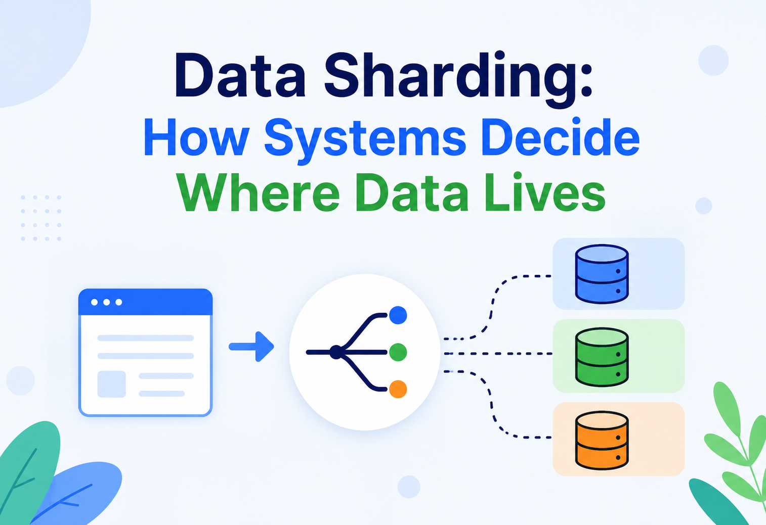
Data Sharding: How Systems Decide Where Data Lives?
Range, hash, consistent hashing, directory‑based, and geographic strategies — explained from first principles to production practice, with worked Java code, sequence diagrams, and real stories from Instagram, DynamoDB, Spanner, Facebook, Slack, and YouTube.
Introduction & A Short History
Imagine a library with a million books. If you tried to put all million books on a single bookshelf, the shelf would collapse. Instead, a smart librarian splits the books across many shelves — maybe by the first letter of the author’s last name, or by subject. Sharding is the same idea, but for databases and data storage.
What is sharding?
Sharding is the practice of splitting a large dataset into smaller, more manageable pieces called shards, and spreading those shards across multiple machines (servers), so that no single machine has to store or process all the data alone.
The hardest and most important question in sharding is not “should we split the data?” — almost everyone agrees splitting is necessary at scale. The real question is:
This tutorial is entirely about answering that one question, in depth, with all the common strategies used in real production systems.
A bit of history
In the early days of computing (1970s‑1990s), most applications ran on a single, powerful server with a single database. This is called vertical scaling — you handle more load by buying a bigger, more powerful machine (more CPU, more RAM, faster disks).
But vertical scaling has a hard ceiling: even the most powerful single server available today cannot handle the scale of something like Google Search, Instagram’s photo storage, or Amazon’s order history. Eventually, you hit a wall where no single machine — no matter how expensive — is enough.
This gave rise to horizontal scaling: instead of one giant machine, you use many smaller (and cheaper) machines working together. Sharding is the technique that makes horizontal scaling possible for data specifically — because a database needs to know exactly where each piece of data lives, even when it is spread across hundreds or thousands of machines.
The concept became mainstream in the 2000s and 2010s as companies like Google (Bigtable, Spanner), Amazon (DynamoDB), and Facebook (Cassandra, originally built at Facebook) needed to handle web‑scale data that no single database server could hold.
A simple analogy for everyone
Imagine a school with 1,000 students, but only enough classroom space for 50 students per room. The school needs a rule for which student goes into which classroom. Some possible rules: alphabetical by last name (A‑E in Room 1, F‑J in Room 2, and so on); by grade level (all 3rd graders in Room 1, all 4th graders in Room 2); or randomly assigned, but recorded in a big notebook so the school always knows which room a student is in. Each of these rules is a different sharding strategy — and just like in real databases, each has trade‑offs (what happens when a new student joins? What if one classroom becomes overcrowded?).
Problem & Motivation
Before deciding how to shard, it helps to feel why a growing application eventually has to split its data at all.
Why do we need to split data at all?
As an application grows, it runs into limits:
Storage limits
A single disk or server can only hold so much data (measured in terabytes, not infinite).
Throughput limits
A single database server can only handle so many reads / writes per second before it becomes the bottleneck.
Memory limits
Indexes and caches need to fit in RAM for fast access; a huge dataset will not fit in one machine’s memory.
Geographic latency
Users in Japan should not have to wait for a database server sitting in Virginia, USA, for every single request.
Sharding solves all four problems by spreading data (and the corresponding load) across many machines.
The core motivation: the sharding‑key decision
Once you decide to split your data, you must decide: what determines which shard a specific row / record goes to? This decision is driven by something called the shard key (also called a partition key).
A specific field (or combination of fields) in your data — like user_id, country, or order_id — that is used to determine which shard a piece of data belongs to.
Why this matters so much: pick the wrong shard key, and you can end up with:
- Hot shards (one shard gets overloaded while others sit nearly idle) — like one classroom with 500 students while others have 5.
- Difficult queries (needing to search every shard to answer a simple question, defeating the purpose of sharding).
- Painful re‑sharding (having to move massive amounts of data around when you add more machines).
This tutorial focuses on the common strategies for making this shard‑key decision correctly.
Core Concepts
Every conversation about sharding uses the same handful of nouns. Nailing them down here saves confusion later.
Shard
A shard is one independent, self‑contained slice of the overall dataset, typically stored on its own server (or its own dedicated storage / database instance). Analogy: one classroom in our school example. Practical example: in a system with 4 shards, Shard-0, Shard-1, Shard-2, Shard-3 each might hold roughly 25% of all user records.
Shard key (partition key)
The field(s) used to decide shard placement. Why it exists: without a defined rule, there is no consistent way to find data later. If you do not know the rule for where a student sits, you cannot find them again either. Practical example: in an e‑commerce system, you might shard the orders table by customer_id — meaning all orders belonging to the same customer always land in the same shard.
Partitioning vs sharding (clarifying confusing terms)
These terms are often used interchangeably, but there is a subtle distinction worth knowing:
- Partitioning is the general concept of splitting data into parts — this can happen within a single machine too (e.g., splitting one huge table into smaller partitions on the same server, by date range, for easier management).
- Sharding specifically refers to partitioning data across multiple separate machines / servers (horizontal scaling), where each shard usually runs as an independent database instance.
So: all sharding is a form of partitioning, but not all partitioning is sharding. Many database systems (like PostgreSQL) support “table partitioning” on a single server as a stepping stone before full sharding across multiple servers.
Routing layer
The routing layer (sometimes called a “shard router” or “proxy”) is the piece of software that looks at an incoming request, figures out which shard the relevant data lives on, and sends the request to that shard. Analogy: the school receptionist who, when a parent calls asking about their child, checks the notebook and says, “Your child is in Room 3, let me connect you.” Practical example: in MongoDB’s sharded clusters, a component called mongos acts as this routing layer.
Rebalancing / resharding
Rebalancing is the process of moving data between shards — usually because shards have become uneven in size or load, or because new shards were added to the cluster. Why it exists: data grows unevenly over time. A shard key that seemed balanced on day one might become lopsided a year later (e.g., if your platform suddenly gets popular in one specific country). Analogy: moving some students from an overcrowded classroom to a newly opened classroom down the hall.
Hot shard / hotspot
A hot shard is a shard that receives disproportionately more traffic or data than the others, becoming a bottleneck even though the overall system has plenty of spare capacity elsewhere. Analogy: one classroom with 200 students crammed in, while nine other classrooms sit half‑empty — the school “as a whole” has room, but that one room is still a fire hazard. Practical example: if you naively shard a social media app’s data by country, and 60% of your users are in the USA, the “USA shard” becomes extremely hot while smaller countries’ shards stay nearly empty.
Architecture & Components
A sharded database has more moving parts than a single one. Here is the picture, then the parts.
Diagram explanation: the client never talks to shards directly. It talks to a routing layer, which uses the shard key (here, user_id = 12345) plus a sharding strategy (here, hashing) to figure out exactly which shard holds this data, then forwards the request only to that shard. A separate metadata store keeps track of which shard is responsible for which range / hash of keys — this metadata is critical and must itself be highly available (if it goes down, the whole routing system is blind).
Key components
Extracts the key
The logic that extracts the shard key from a request (e.g., pulling user_id out of an incoming API call).
Maps key to shard
The algorithm that maps a shard key to a specific shard (hashing, ranges, or a lookup directory — covered in detail in Chapter 5).
Sends the request
Directs requests to the correct shard based on the strategy’s output.
Authoritative map
Keeps the authoritative record of shard boundaries / assignments — often itself a small, highly‑available, strongly‑consistent database (ironic, but necessary).
The actual data
The actual databases / storage nodes holding the real data.
Background orchestrator
A background process that monitors shard sizes / load and triggers data migration when needed.
Internal Working — Common Strategies for Deciding How to Shard
This is the heart of the tutorial. Let us go through each major strategy, step by step.
Strategy 1 — Range‑Based (Range Partitioning) Sharding
What it is: data is split into shards based on ranges of the shard key’s value. For example, if sharding by user_id:
- Shard 0:
user_id1 – 1,000,000 - Shard 1:
user_id1,000,001 – 2,000,000 - Shard 2:
user_id2,000,001 – 3,000,000
Why it exists: it is simple to understand and implement, and it makes range queries (e.g., “give me all orders from January to March”) efficient, because a contiguous range of data lives together on the same shard(s).
Sorting library books alphabetically by author’s last name onto different shelves: A‑F on Shelf 1, G‑M on Shelf 2, and so on.
Beginner example: a school assigning classrooms based on student ID number ranges: IDs 1‑100 in Room A, 101‑200 in Room B. Software example: sharding a time_series table of sensor readings by date range — all of January’s data on Shard 1, all of February’s data on Shard 2. This is extremely common for logging and time‑series databases. Production example: Google’s Bigtable and Apache HBase use range‑based partitioning of their key space by default, which is why they are well‑suited for time‑ordered or lexicographically‑ordered data (like web crawl data sorted by domain name).
Step‑by‑step working
Boundary table maintained
The system maintains a small lookup table describing shard boundaries (e.g., “Shard 0 covers keys A000000 to A999999”).
Compare on request
When a request comes in with a shard key, the routing layer does a simple comparison against these boundaries to determine the shard.
Split as data grows
As data grows, a range can be split into two smaller ranges (and its shard split into two shards) when it grows too large.
Advantages
- Efficient range queries (e.g., “all events between two dates”).
- Simple to reason about and debug.
- Easy to add new shards at the “end” of the range (e.g., new user IDs just go to a new shard).
Disadvantages
- Hotspotting risk: if data is inserted in increasing order (like auto‑incrementing IDs or timestamps), all new writes go to the same, most recent shard — creating a severe hot shard while older shards go completely idle. This is one of the most well‑known pitfalls in sharding.
- Requires ongoing management of range boundaries as data grows unevenly.
Strategy 2 — Hash‑Based Sharding
What it is: the shard key is passed through a hash function — a mathematical function that converts any input into a fixed‑size, seemingly random‑looking number — and the result determines the shard, typically using a modulo operation.
shard_number = hash(shard_key) % number_of_shardsWhat is a hash function? It is a function that takes any input (a string, a number, anything) and produces a fixed‑size output (like a 32‑bit or 64‑bit number), designed so that even tiny changes in input produce very different‑looking outputs, and so that outputs are spread evenly across the possible range (this property is called good “distribution” or “avalanche effect”).
Why it exists: unlike range‑based sharding, hashing spreads data (and therefore load) evenly and unpredictably across all shards, avoiding the “all new data in one shard” hotspot problem.
Instead of sorting library books alphabetically (which might overload the “S” shelf because so many authors’ last names start with S), you assign each book a random shelf number based on a scrambling formula applied to its ISBN — spreading books evenly no matter what letter they start with.
Beginner example: suppose you have 4 shards and a shard key of user_id. hash(12345) % 4 = 1 → this user’s data goes to Shard 1. hash(67890) % 4 = 3 → this user’s data goes to Shard 3. Software example: many NoSQL databases (like MongoDB’s hashed sharding, or Cassandra’s default partitioner) use this approach for exactly this reason — to spread writes evenly. Production example: Amazon’s DynamoDB uses hash‑based partitioning on the “partition key” of every table by default, specifically to avoid hotspots and provide predictable, even performance regardless of data patterns.
Java example — hash‑based shard selection
// Simple demonstration of hash-based shard selection in Java
public class HashShardRouter {

    private final int numberOfShards;

    public HashShardRouter(int numberOfShards) {
        this.numberOfShards = numberOfShards;
    }

    public int getShardFor(String shardKey) {
        // Use a well-distributed hash function (never rely on Java's
        // default hashCode() alone in production - it's not guaranteed
        // stable across JVM versions for all types).
        int hash = Math.abs(murmurHash(shardKey));
        return hash % numberOfShards;
    }

    // Simplified illustrative hash (in production, use a library
    // like Guava's Hashing.murmur3_32() or a similar vetted implementation)
    private int murmurHash(String key) {
        int h = 0;
        for (char c : key.toCharArray()) {
            h = 31 * h + c;
        }
        return h;
    }

    public static void main(String[] args) {
        HashShardRouter router = new HashShardRouter(4);
        System.out.println("user_12345 -> Shard " + router.getShardFor("user_12345"));
        System.out.println("user_67890 -> Shard " + router.getShardFor("user_67890"));
        System.out.println("user_11111 -> Shard " + router.getShardFor("user_11111"));
    }
}
Explanation: the getShardFor method takes any shard key (here, a user identifier as a string), runs it through a hash function, and takes the result modulo the number of shards. Because a good hash function scatters similar‑looking inputs into very different outputs, sequential or similar keys (like user_12345 and user_12346) usually land on completely different shards, avoiding the “hot recent shard” problem seen in naive range sharding.
Advantages
- Even data / load distribution — no hotspotting from sequential keys.
- Simple to implement and reason about for single‑key lookups.
Disadvantages
- Range queries become expensive: hashing scrambles the natural order of keys, so a query like “give me all orders from January” now has to check every single shard, since January’s orders are scattered randomly across all of them (called a scatter‑gather query).
- Adding / removing shards is painful: if you go from 4 shards to 5, the modulo operation (
hash(key) % 5vshash(key) % 4) produces completely different results for almost every key — meaning almost all data needs to be physically moved to new shards. (Consistent hashing, covered next, solves this specific problem.)
Strategy 3 — Consistent Hashing
What it is: an improved hashing technique specifically designed to minimise data movement when shards are added or removed. Why it exists: as explained above, plain hash‑based sharding (hash(key) % N) causes almost all data to be reshuffled when N (the number of shards) changes. Consistent hashing was invented (originally by researchers at MIT in 1997, for early web caching systems, and later popularised by Amazon’s Dynamo paper in 2007) to solve exactly this pain point.
How it works, step by step
Imagine a ring
A circle representing all possible hash values, from 0 up to some very large maximum number, wrapping back around to 0 (like a clock face, but with billions of positions instead of just 12).
Place each shard on the ring
Each shard (server) is placed at one or more points on this ring, based on hashing the shard’s own identifier (like its server name or IP address).
Place each key on the ring
Each piece of data is also hashed, placing it at a point on the same ring.
Walk clockwise
To find which shard owns a piece of data, you move clockwise around the ring from the data’s position until you hit the first shard.
The key benefit
When a new shard is added, it only takes over a small slice of the ring (the portion between it and the next shard counter‑clockwise) — meaning only a small fraction of data needs to move, not everything.
Diagram explanation: shards are placed at specific positions around a circular hash space. Any piece of data is assigned to the next shard found clockwise from its own hashed position. If a new shard were inserted at position 50, it would only “steal” data that currently falls between position 20 (Shard A) and 50 — a small slice previously owned by Shard B — leaving all other shards’ data completely untouched.
Imagine assigning classrooms not by a simple number range, but by placing each classroom door at a specific point around a circular hallway, and telling each student, “Walk clockwise from your assigned starting spot in the hallway, and enter the very first classroom door you reach.” If you add one new classroom door into the hallway, only the students who would have walked past that exact spot are affected — everyone else’s assigned classroom stays exactly the same.
Practical / production example: Amazon’s Dynamo (and its open‑source descendant, Apache Cassandra) uses consistent hashing internally to place data across nodes, specifically so that adding or removing servers causes minimal data reshuffling — critical for a system designed to run continuously with rolling hardware changes and failures.
Virtual nodes (an important refinement)
In practice, each physical shard is usually given many positions on the ring (called virtual nodes or “vnodes”) rather than just one, because a single random position per shard can lead to uneven ring coverage (some shards ending up responsible for much bigger arcs of the ring than others, purely by chance). Using, say, 100‑256 virtual nodes per physical shard smooths this out, giving a much more even distribution.
Advantages
- Minimal data movement when scaling the cluster up or down.
- Naturally supports gradual, incremental scaling — a huge operational win compared to plain modulo hashing.
Disadvantages
- More complex to implement and reason about than simple modulo hashing.
- Still suffers from the same range‑query weakness as plain hashing (data order is not preserved).
Strategy 4 — Directory‑Based (Lookup Table) Sharding
What it is: instead of computing which shard owns a key via a formula (hash or range), the system maintains an explicit lookup table (a directory) that records, for every key (or group of keys), exactly which shard it lives on.
Why it exists: sometimes the “right” shard for a piece of data depends on business logic that a formula cannot easily capture — for example, you might want to keep a specific big customer’s data on its own dedicated, more powerful shard for compliance or performance reasons, regardless of what a hash function would say.
Instead of a fixed rule like “alphabetical” or “random assignment,” the school secretary keeps an actual notebook: “Emma Johnson → Room 3. David Lee → Room 7.” Placement decisions can be made individually, for any reason.
Beginner example: a very small startup with 3 big enterprise clients might keep a simple mapping: Client A → Database Server 1, Client B → Database Server 2, Client C → Database Server 3. Software example: multi‑tenant SaaS platforms often use a directory / lookup approach, mapping each tenant_id to a specific shard, recorded in a small, separate “tenant metadata” database. Production example: Instagram’s early sharding system (before their move to more sophisticated custom ID generation) and many large multi‑tenant B2B platforms (like Salesforce’s “pod” architecture) use directory‑based approaches, allowing operators to manually move a specific busy customer to a dedicated, larger shard when needed.
Step‑by‑step working
Maintain a lookup directory
A lookup table (directory) is maintained, typically in its own small, fast, highly‑available database (since every single request depends on checking it first).
Look up on each request
On each request, the routing layer looks up the shard key in the directory to find the assigned shard.
Update entries as needed
Administrators (or automated rebalancing tools) can update individual entries in the directory to move specific keys to different shards, without affecting anyone else.
Advantages
- Maximum flexibility — any custom placement logic is possible (e.g., isolating a noisy customer, complying with data residency laws by region, giving VIP customers dedicated resources).
- Rebalancing can be done key‑by‑key, very granularly, without a big “recompute everything” event.
Disadvantages
- Extra lookup cost: every single request needs an additional lookup step before it even knows which shard to talk to — this directory itself must be extremely fast and highly available, or it becomes a bottleneck and single point of failure for the entire system.
- Operational overhead: someone (or some automated system) has to actively maintain and update this directory as data grows — it does not “just work” via a mathematical formula.
Strategy 5 — Geographic / Attribute‑Based Sharding
What it is: data is sharded based on a meaningful real‑world attribute — most commonly geographic region (e.g., US-shard, EU-shard, Asia-shard), but also possibly by customer tier, product category, or business unit.
Why it exists: beyond pure load balancing, there are often legal, regulatory, and latency reasons to keep certain data physically located in specific places. For example, the EU’s GDPR (General Data Protection Regulation) and similar data‑residency laws in other countries often require that certain user data physically stay within specific national or regional borders.
A multinational company keeping separate, local filing cabinets in each country’s office, both because it is faster for local staff to access nearby files, and because some countries legally require certain records to never leave the country.
Beginner example: a photo‑sharing app storing European users’ photos on servers physically located in Europe, and American users’ photos on servers in the US. Production example: major cloud‑based SaaS platforms and social media companies (Facebook / Meta, TikTok, and others) shard significant portions of user data by geographic region, both for latency (serving users from a nearby data centre) and for regulatory compliance with regional data laws.
Advantages
- Naturally satisfies legal / regulatory data residency requirements.
- Improves latency for geographically distributed users (data is physically closer to them).
Disadvantages
- Can create uneven shard sizes if user populations are very unevenly distributed across regions (e.g., far more users in one country than another) — often combined with hash‑based sharding within each region to smooth this out.
- Cross‑region queries or a user travelling / moving between regions can add complexity.
Combining strategies (hybrid approaches)
In real production systems, it is extremely common to combine these strategies. For example:
- Shard first by geographic region (for compliance / latency), then apply consistent hashing within each region’s cluster (for even load distribution).
- Use directory‑based overrides for a small number of special, high‑value customers, while using hash‑based sharding as the default for everyone else.
This layered approach captures the benefits of multiple strategies while managing their individual weaknesses.
Data Flow & Lifecycle
Every read and every write in a sharded system follows the same short dance: figure out the shard, then forward the request. Here is what that looks like end to end.
Lifecycle of data as a system scales
Initial design
Choose a shard key and strategy based on expected query patterns and data growth.
Steady state
Data flows in and out of shards according to the chosen strategy.
Monitoring
Track per‑shard size, CPU / memory usage, and query latency to detect emerging hotspots.
Rebalancing trigger
When a shard grows too large or too busy, a rebalancing process kicks off.
Migration
Data is copied (and eventually cut over) from an overloaded shard to a new or less‑busy shard, ideally with minimal downtime (often using techniques like dual writes during migration, followed by a verified cutover).
Cleanup
Old, now‑unused copies of migrated data are deleted from their original shard.
Advantages, Disadvantages & Trade‑Offs
The strengths and weaknesses of sharding — and a side‑by‑side view of how the five strategies compare on the properties that matter most.
General sharding advantages
| Advantage | Explanation |
|---|---|
| Horizontal scalability | Add more machines to handle more data / traffic, instead of hitting a hard single‑server ceiling |
| Improved performance | Smaller datasets per shard mean faster queries and smaller indexes that fit better in memory |
| Fault isolation | A failure in one shard does not necessarily bring down the entire dataset — other shards keep working |
| Parallelism | Queries that can be split across shards can run in parallel, finishing faster overall |
General sharding disadvantages
| Disadvantage | Explanation |
|---|---|
| Increased complexity | Application code, routing logic, and operations all become more complicated than a single database |
| Cross‑shard queries are hard | Joining or aggregating data across multiple shards (e.g., “total sales across all customers”) requires special handling — often a “scatter‑gather” pattern that queries every shard and merges results |
| Cross‑shard transactions are hard | Keeping data consistent when a single logical operation spans multiple shards (e.g., transferring money between two users on different shards) requires distributed transaction protocols (like two‑phase commit) or careful application‑level design |
| Rebalancing overhead | Moving data between shards as the system grows is operationally risky and resource‑intensive |
| Choosing the wrong shard key is costly to fix | Changing your fundamental sharding strategy after the fact, once you have a large amount of data, is one of the most painful migrations in all of software engineering |
Strategy comparison
| Strategy | Even Load Distribution | Range Query Support | Data Movement on Resize | Complexity |
|---|---|---|---|---|
| Range‑based | Poor (hotspot risk) | Excellent | Moderate | Low |
| Hash‑based (modulo) | Excellent | Poor | Very High | Low – Medium |
| Consistent hashing | Excellent | Poor | Low | Medium – High |
| Directory‑based | Depends on rules | Depends on rules | Low (granular) | Medium (extra lookup) |
| Geographic / attribute | Depends on population | Good within region | Low | Medium |
Performance & Scalability
The single biggest performance factor in sharding is shard‑key selection, and it should be based on your actual query patterns, not just convenience.
Choosing a shard key — the real performance decision
What is the most common access pattern?
If 95% of queries fetch data by user_id, then user_id is likely your shard key — this ensures the vast majority of queries hit exactly one shard (called being shard‑local or single‑shard queries), which is by far the fastest and cheapest kind of query.
Does the key have high cardinality?
A shard key like is_premium_user (only two possible values: true / false) is a terrible shard key — it can only ever create two shards, no matter how many machines you add. A shard key like user_id (millions of distinct values) allows fine‑grained, scalable distribution.
Will the key cause hotspots?
Sequential / monotonically increasing keys (like auto‑incrementing IDs or timestamps) are dangerous with range‑based sharding, because all new writes concentrate on the newest shard.
Scatter‑gather queries and their cost
When a query cannot be satisfied by a single shard (e.g., “find the top 10 most active users across the entire platform”), the system must:
Scatter
Send the query to every shard.
Wait
Wait for all shards to respond.
Gather
Combine and re‑sort the partial results from each shard into one final answer.
The overall query latency is bound by the slowest shard’s response time (not the average), and this pattern puts load on every shard for every such query, defeating some of the isolation benefits of sharding. Good schema / shard‑key design tries to minimise how often scatter‑gather queries are needed.
Read replicas within shards
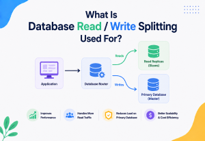
It is common to combine sharding (splitting data horizontally across machines) with replication (having copies of each shard for read scaling and fault tolerance). Each shard might have one primary (handles writes) and several read replicas (handle read traffic), multiplying the total read capacity without needing more shards.
High Availability & Reliability
Sharding on its own only handles scale. Reliability comes from combining sharding with replication — and from taking the metadata store as seriously as the shards themselves.
Replication within each shard
Every shard should itself be replicated (typically 3 copies is a common industry default) so that the failure of a single machine does not cause data loss or an outage for that shard’s slice of data. This combines two distinct concepts:
- Sharding: spreads different data across different machines (for scale).
- Replication: keeps copies of the same data on multiple machines (for reliability).
Modern distributed databases (Cassandra, MongoDB, CockroachDB, Google Spanner) apply both simultaneously — every shard is itself a small replicated cluster.
Diagram explanation: each shard is not a single point of failure — it is internally a small cluster with a primary and replicas. If the primary of Shard 0 fails, one of its replicas is promoted to become the new primary, and Shard 0 continues serving its slice of data with minimal interruption.
Shard metadata availability
The shard metadata store (which tracks where each shard’s boundaries / assignments live) is arguably the most critical piece of the entire architecture — if it becomes unavailable or returns incorrect information, requests cannot be routed correctly anywhere in the system, even if every individual shard is perfectly healthy. This is why metadata stores typically use strongly consistent, highly available consensus‑based systems (like ZooKeeper, etcd, or a small dedicated consensus cluster) rather than a single simple server.
Failure recovery considerations
- Single shard failure: with proper replication, a single shard node failure is transparent to users — a replica takes over.
- Whole shard unreachable (network partition): depending on the consistency model chosen (see CAP theorem in Chapter 18), the system may either become temporarily unavailable for that shard’s data, or serve slightly stale data, to keep functioning.
- Backup and disaster recovery: each shard needs its own backup strategy (typically automated periodic snapshots plus continuous write‑ahead‑log shipping), since a full dataset restore now means restoring many independent shards consistently, not just one database.
Security
Sharding meaningfully changes the security picture — sometimes for the better (isolation), sometimes for the worse (more moving parts to lock down).
Per‑tenant data isolation
In multi‑tenant systems using directory‑based sharding, keeping different customers’ data on physically separate shards can be a strong security / compliance boundary — a bug in query logic is less likely to leak Customer A’s data into Customer B’s results if they are on entirely separate database instances.
Data residency
As discussed, geographic sharding directly supports legal requirements (GDPR in Europe, data localisation laws in countries like Russia, China, and India) by guaranteeing that specific data never leaves specific physical / legal jurisdictions.
Per‑shard authentication
Each shard should enforce its own authentication and authorisation, and the routing layer should never expose raw shard connection details to end clients — clients should only ever talk to the routing layer / application layer, never directly to individual shard databases.
In transit and at rest
Data should be encrypted both in transit (between the routing layer and shards, using TLS) and at rest (on each shard’s storage), consistently across all shards — a common security mistake is to apply strong encryption to some shards but forget newly added ones.
Monitoring, Logging & Metrics
Sharded systems need monitoring per‑shard, not just in aggregate, because problems often hide behind healthy‑looking averages.
| Metric | Why it matters |
|---|---|
| Per‑shard storage size | Detects shards growing disproportionately large (candidates for splitting) |
| Per‑shard query rate (QPS) | Detects hot shards receiving disproportionate traffic |
| Per‑shard latency (p50 / p95 / p99) | A single slow shard can drag down scatter‑gather queries across the whole system |
| Cross‑shard query ratio | Tracks how often expensive scatter‑gather queries occur vs. efficient single‑shard queries — a rising ratio suggests the shard key may need reconsideration |
| Rebalancing / migration progress | Tracks ongoing data movement operations, which can be resource‑intensive and need careful monitoring |
| Shard metadata store health | Since this is a single point of failure for routing, it needs its own dedicated, high‑priority monitoring |
A dashboard showing “data size per shard” as a bar chart is one of the fastest ways to visually spot an imbalance — if one bar is dramatically taller than the rest, that is your hot shard, and it is time to investigate the shard key or trigger a rebalance.
Deployment & Cloud
Modern cloud providers offer managed solutions that handle much of the sharding complexity automatically — here are the ones you will hear about most often, and the deployment habits that keep them healthy.
Managed sharding services
Invisible partitioning
Fully managed, hash‑based partitioning is automatic and invisible to the developer — you simply choose a good partition key, and AWS handles routing, rebalancing, and replication behind the scenes.
Range + strong consistency
Uses range‑based sharding internally but with sophisticated automatic splitting and load‑based rebalancing, while still providing strong consistency and even cross‑shard transactions (a major engineering achievement, covered more in Chapter 18).
Range or hashed clusters
Supports both range‑based and hash‑based sharding, with the mongos routing layer and config servers (metadata store) as distinct, explicitly managed components.
Sharding middleware for MySQL
An open‑source sharding middleware layer built on top of MySQL, adding sharding, connection pooling, and query routing to standard MySQL databases without changing the underlying database engine. Used by YouTube, Slack, and others.
Deployment best practices
- Deploy shard metadata stores across multiple availability zones for high availability, since it is a critical single point of failure if not properly replicated.
- Plan capacity for at least one full shard’s worth of headroom, so you can always add a new empty shard for rebalancing without first needing to free up space.
- Automate rebalancing where possible, but always with monitoring / alerting and the ability to pause or roll back a migration if something goes wrong mid‑way.
- Use infrastructure‑as‑code (Terraform, CloudFormation) to keep shard provisioning consistent and repeatable, especially as the number of shards grows into the dozens or hundreds.
Databases, Caching & Load Balancing
Caches are sharded too. And load balancing in a sharded architecture is meaningfully different from stateless load balancing, because the choice of destination is dictated by data, not just by picking the least‑busy server.
Sharding‑aware caching
Caches (like Redis) are often sharded using the exact same strategies discussed here (commonly consistent hashing, since Redis Cluster itself uses a hash‑slot mechanism internally — 16,384 fixed hash slots distributed across nodes, a practical, simplified variant of consistent hashing). This ensures cache lookups can be routed efficiently, just like database lookups.
Java example — Redis‑Cluster‑style hash slot assignment
// Simplified illustration of Redis-Cluster-style hash slot assignment
public class HashSlotRouter {
    private static final int TOTAL_SLOTS = 16384; // Redis Cluster's fixed slot count

    public int getSlotFor(String key) {
        int hash = crc16(key) % TOTAL_SLOTS;
        return hash;
    }

    // Simplified stand-in; real Redis Cluster uses CRC16 specifically
    private int crc16(String key) {
        int crc = 0;
        for (char c : key.toCharArray()) {
            crc = (crc << 5) - crc + c;
        }
        return Math.abs(crc);
    }
}
Explanation: every key is mapped to one of 16,384 fixed “slots,” and each slot is assigned to a specific node. This fixed‑slot approach is a practical middle ground: it gives most of consistent hashing’s benefits (minimal movement when nodes change) while being simpler to implement and reason about, since the slots (not individual keys) are what get reassigned to nodes.
Load balancing across shards
Load balancers in a sharded architecture typically work at the routing‑layer level — directing traffic not just to “any healthy server” (as in a simple stateless web app) but specifically to the correct shard for each request. This is fundamentally different from traditional load balancing, since the choice of destination is determined by data, not just by picking the least‑busy available server.
APIs & Microservices
Sharding shows up inside microservices too — and a well‑designed API keeps clients blissfully unaware of it.
Database‑per‑service with internal sharding
In a microservices architecture, it is common for each service to own its own database (the “database‑per‑service” pattern), and for that individual database to itself be sharded if that particular service handles very high volume (e.g., an “Orders” service at a large e‑commerce company might have its own dedicated, heavily sharded database, while a smaller “Settings” service uses a single, unsharded database).
Exposing shard keys through APIs
A well‑designed API should generally hide sharding details from clients entirely — a client calling GET /users/12345 should not need to know or care that user 12345’s data physically lives on “Shard 7.” The routing logic should be entirely internal, encapsulated behind the API layer. However, the API design can subtly encourage efficient sharding by requiring the shard key as part of common request patterns (e.g., requiring both customer_id and order_id in requests, so lookups are always shard‑local rather than requiring a wasteful scatter‑gather).
Design Patterns & Anti‑Patterns
A handful of patterns keep showing up in mature sharded systems — and an equally recognisable handful of anti‑patterns show up in the ones that struggle.
Good design patterns
Shard key aligned with access pattern
Always choose the shard key based on your most frequent, latency‑sensitive queries.
Consistent hashing with virtual nodes
The modern default choice for systems needing even load distribution and easy scaling.
Denormalisation for shard locality
Sometimes duplicating a small piece of data (e.g., storing a copy of customer_name alongside every order) avoids needing a cross‑shard join just to display a name — trading some storage / consistency overhead for major query simplicity.
Fan‑out with an aggregation service
For necessary cross‑shard queries, build a dedicated aggregation service that handles the scatter‑gather pattern cleanly, rather than scattering this logic across every part of the application.
Anti‑patterns to avoid
Low‑cardinality shard key
Fields like boolean flags or small fixed categories (status: active / inactive) make terrible shard keys because they cap how many shards you can ever meaningfully have.
Monotonic keys + range partitioning
Causes severe hotspotting on the newest shard — a very common real‑world mistake, especially with auto‑incrementing primary keys.
Ignoring cross‑shard transactions
Discovering after going live that a core business operation (like “transfer funds between two accounts”) frequently spans two different shards, without having designed for it, leads to painful, risky retrofits.
Aggregate‑only monitoring
Aggregate metrics hide exactly the kind of imbalance sharding is meant to help you manage — one of the most common operational blind spots.
Strategy chosen before query patterns
Picking hash‑based sharding “because it is popular,” without checking whether your application desperately needs efficient range queries (which hash‑based sharding makes expensive), is a common and costly mistake.
Best Practices & Common Mistakes
Turning the theory into durable operational habits.
Best practices
Choose your shard key based on real, measured query patterns
Not guesses. Not “whatever field is available.” Actual measured traffic.
Prefer high‑cardinality shard keys
Fields with many distinct values naturally spread load; low‑cardinality fields cannot.
Default to consistent hashing (with virtual nodes)
Use it for hash‑based sharding unless you have a specific reason to use plain modulo hashing.
Combine sharding with replication
Sharding alone does not provide fault tolerance. Every shard should itself be replicated.
Monitor per‑shard metrics
System‑wide averages hide the exact imbalances sharding is meant to expose.
Design to minimise cross‑shard queries
Design your application to minimise cross‑shard queries and transactions from the start.
Plan and test rebalancing early
Practise your rebalancing / resharding process before you desperately need it under production pressure.
Consider a managed service
Consider DynamoDB, Spanner, Vitess, or MongoDB Atlas rather than building custom sharding logic from scratch unless you have a very specific, unmet need.
Common mistakes
- ✗ Treating shard key selection as an afterthought, then discovering hotspots only after a painful production incident.
- ✗ Forgetting that a “cross‑shard join” is now a distributed‑systems problem, not a simple SQL
JOIN— and not planning for it. - ✗ Under‑provisioning the shard metadata store, treating it as an unimportant detail even though it is a critical single point of failure.
- ✗ Failing to test rebalancing / migration procedures at realistic data volumes before relying on them in production.
- ✗ Assuming sharding alone solves availability problems — without replication within each shard, sharding actually increases your total number of potential failure points, since you now depend on many machines being up instead of just one.
Real‑World & Industry Examples
How some of the biggest platforms in the world actually shard their data — and the specific technical choices they became known for.
Shard number inside the ID
In Instagram’s early growth, they famously built a custom ID generation scheme, encoding the shard number directly into every generated ID (using bit‑shifting: part of each 64‑bit ID represents a timestamp, part represents the shard number, and part is a per‑shard counter). This meant that just by looking at a photo’s ID, their systems immediately knew which shard to query — no separate lookup or hashing step needed at read time. A clever hybrid: essentially a form of directory‑based sharding baked directly into the identifier itself.
Dynamo paper heritage
DynamoDB uses hash‑based partitioning as its foundational design, guided by Amazon’s own influential 2007 “Dynamo” research paper, which introduced (or heavily popularised) consistent hashing for large‑scale, highly available key‑value storage. This heritage directly shaped how an entire generation of NoSQL databases (Cassandra, Riak, Voldemort) approached sharding.
Range + TrueTime
Google Spanner is notable for offering range‑based sharding combined with strong consistency and even distributed, cross‑shard ACID transactions — historically considered extremely difficult to achieve together at global scale. It does this using a specialised technology called TrueTime (leveraging atomic clocks and GPS receivers in Google’s data centres) to precisely order transactions across shards spread around the entire globe.
MySQL at massive scale
Facebook historically sharded enormous MySQL deployments using techniques very similar to directory‑based sharding for its social‑graph data, combined with extensive caching (Memcached) in front of the sharded databases to absorb read load — a pattern widely copied across the industry afterward.
Vitess middleware for MySQL
Both Slack and YouTube use (or have used) Vitess, an open‑source sharding middleware for MySQL originally built at YouTube, which adds automated, consistent‑hashing‑based sharding on top of standard, familiar MySQL databases — letting these companies scale MySQL horizontally without rewriting their applications to use an entirely different database technology.
Advanced Topics
The deeper distributed‑systems ideas that sharding forces teams to reckon with, and a production‑shape implementation of the consistent hashing ring.
CAP theorem and sharding
The CAP theorem states a distributed system can only fully guarantee two of these three properties during a network partition: Consistency, Availability, and Partition Tolerance. Sharded systems are inherently distributed, so this theorem directly applies:
- If a shard becomes network‑partitioned from the rest of the system, the system must choose: serve possibly‑stale data from that shard (favouring Availability), or refuse to serve requests to that shard’s data until the partition heals (favouring Consistency).
- Systems like Cassandra typically favour availability (an “AP” system in CAP terms) by default, allowing configurable consistency levels per query. Systems like Google Spanner aim for very strong consistency (“CP”‑leaning) using extremely precise time synchronisation to minimise the practical impact of this trade‑off.
Distributed transactions across shards
When a single logical operation needs to update data on two different shards atomically (e.g., moving money from Account A on Shard 1 to Account B on Shard 2), simple single‑database transactions no longer work. Common solutions:
- Two‑Phase Commit (2PC): a coordinator asks all involved shards to “prepare” the transaction (locking relevant data and confirming they can commit), and only after all shards confirm readiness does it tell them all to actually “commit.” If any shard fails to prepare, the whole transaction is aborted everywhere. Downside: it can block if the coordinator crashes mid‑process, and it reduces overall system availability during the transaction window.
- Saga Pattern: instead of a single atomic transaction, the operation is broken into a sequence of smaller, independent local transactions, each with a defined “compensating action” to undo it if a later step fails (e.g., “reverse the debit from Account A” if the credit to Account B fails). This trades strict atomicity for better availability and is very popular in modern microservices architectures.
Diagram explanation: because the debit and credit happen on two different shards, they cannot be wrapped in one simple database transaction. The Saga pattern instead performs each step separately, and if a later step fails, it runs a “compensating” action to undo the earlier, already‑completed step — ensuring the overall system ends up in a consistent state, even without true cross‑shard atomicity.
Replication strategies combined with sharding
- Single‑leader replication per shard: each shard has one primary (accepting writes) and multiple followers / replicas (serving reads) — the most common approach (used by MySQL, PostgreSQL‑based sharded systems).
- Leaderless replication: used by Cassandra and DynamoDB, where any replica can accept writes, and conflicts are resolved using techniques like “last write wins” or vector clocks — offering higher write availability at the cost of more complex conflict resolution.
Consensus algorithms for shard metadata
Since the shard metadata store is so critical, it typically uses a consensus algorithm (like Raft or Paxos) internally to ensure all nodes of the metadata store agree on the current shard assignments, even if some metadata nodes fail or become temporarily unreachable. Tools like etcd (which uses Raft) and Apache ZooKeeper (which uses a Paxos‑like protocol called ZAB) are commonly used specifically for this purpose in real sharded systems (e.g., Kubernetes itself uses etcd for its own cluster state, a similar problem to shard metadata management).
Data structures: consistent hashing ring implementation details
A production consistent‑hashing implementation typically uses a sorted data structure (like a balanced binary search tree, or a sorted array with binary search) to represent the ring positions of all virtual nodes, enabling an efficient O(log n) lookup (“find the next node clockwise from this hash position”) rather than a slow linear scan through all nodes.
import java.util.TreeMap;

public class ConsistentHashRing {
    private final TreeMap<Long, String> ring = new TreeMap<>();
    private final int virtualNodesPerShard;

    public ConsistentHashRing(int virtualNodesPerShard) {
        this.virtualNodesPerShard = virtualNodesPerShard;
    }

    public void addShard(String shardName) {
        for (int i = 0; i < virtualNodesPerShard; i++) {
            long position = hash(shardName + "-vnode-" + i);
            ring.put(position, shardName);
        }
    }

    public void removeShard(String shardName) {
        ring.entrySet().removeIf(entry -> entry.getValue().equals(shardName));
    }

    public String getShardFor(String key) {
        long hash = hash(key);
        // ceilingEntry finds the next position clockwise (>= hash).
        // If none exists (we've gone past the max), wrap around to the first entry.
        var entry = ring.ceilingEntry(hash);
        if (entry == null) {
            entry = ring.firstEntry();
        }
        return entry.getValue();
    }

    private long hash(String input) {
        // Simplified illustrative hash; production code should use a
        // well-vetted 64-bit hash function like MurmurHash3 or xxHash.
        long h = 1125899906842597L;
        for (char c : input.toCharArray()) {
            h = 31 * h + c;
        }
        return h;
    }
}
Explanation: TreeMap in Java keeps entries sorted by key automatically and supports ceilingEntry(), which efficiently finds the smallest key greater than or equal to a given value — exactly the “walk clockwise to the next shard” operation consistent hashing needs. This gives O(log n) lookup time even with thousands of virtual nodes across many shards, which is essential for a routing layer that must make this decision on every single request without adding noticeable latency.
Failure recovery: shard splitting and merging
- Splitting: when a shard grows too large, it can be split into two smaller shards (common in range‑based systems, where a range like “A‑M” becomes “A‑F” and “G‑M”). This requires careful, often online, data migration to avoid downtime.
- Merging: the reverse operation — combining two under‑utilised shards into one — is less common but sometimes done for cost optimisation when data volume shrinks (e.g., after a data cleanup or archival process).
Frequently Asked Questions
Short, honest answers to the questions that come up almost every time someone new is introduced to sharding.
What is the single most important decision in sharding?
Choosing the shard key. It affects load distribution, query efficiency, and how painful future scaling will be — more than any other single design choice.
Is hash‑based sharding always better than range‑based sharding?
No. Hash‑based sharding avoids hotspots but makes range queries expensive. Range‑based sharding is excellent for range queries but risks hotspotting on sequential keys. The right choice depends entirely on your actual query patterns.
What is consistent hashing solving that plain hashing does not?
Plain hashing (hash(key) % N) requires moving almost all data whenever the number of shards changes. Consistent hashing minimises this data movement to only a small fraction of keys, making it far more practical for systems that grow over time.
Can I change my shard key after going to production?
Technically yes, but it is one of the most expensive and risky migrations in software engineering — it typically requires re‑copying and re‑validating your entire dataset under a new distribution scheme. It is far better to invest time upfront in choosing the right shard key.
Do I need sharding if I only have a few thousand users?
Almost certainly not. Sharding adds real complexity, and a single well‑tuned database server (possibly with read replicas for scaling reads) can handle a surprisingly large amount of load — often millions of rows and thousands of requests per second. Sharding should be introduced when you have clear, measured evidence that a single database can no longer keep up, not preemptively “just in case.”
How is sharding different from replication?
Sharding splits different data across different machines (for scale). Replication keeps copies of the same data across multiple machines (for reliability / read‑scaling). Production systems typically use both together — each shard is itself replicated.
Summary & Key Takeaways
If you remember nothing else from this guide, remember the eight ideas below — and the quiet habit of asking “which shard owns this?” before every design decision that touches data.
Remember This
- Sharding splits a large dataset across multiple machines so no single server has to hold or serve all the data.
- The central challenge is deciding which shard a piece of data belongs to — this is governed by the shard key and a sharding strategy.
- The major strategies are: range‑based (great for range queries, risks hotspots on sequential keys), hash‑based (great for even distribution, poor for range queries), consistent hashing (solves the painful data‑movement problem of plain hashing when scaling), and directory‑based (maximum flexibility, at the cost of an extra lookup and operational overhead).
- Geographic / attribute‑based sharding is often layered on top of these for legal compliance and latency reasons.
- Sharding must be combined with replication for fault tolerance — sharding by itself only addresses scale, not reliability.
- Cross‑shard queries and transactions are fundamentally harder than single‑database operations, requiring patterns like scatter‑gather, two‑phase commit, or the Saga pattern.
- The shard metadata store, though often overlooked, is one of the most operationally critical pieces of the entire system, and typically relies on consensus algorithms (Raft, Paxos) for reliability.
- The golden rule: choose your shard key based on real, measured query patterns, favour high‑cardinality keys, monitor per‑shard health continuously, and plan for rebalancing before you desperately need it.
Sharding is one of the clearest markers of “systems thinking” maturity in software engineering. It sits at the intersection of data modelling, distributed systems theory, and hard‑won operational experience — and understanding it deeply, as covered in this guide, prepares you not just for interviews, but for building and operating real systems at genuine scale.